'Real' FFT    implementation

The previous page illustrated how you can feed real signals in both real and imaginary FFT inputs and later extract the two spectra from the FFT output. The technique is simple, but I want more: feed one real signal into an FFT with length N/2. That is even more convenient in applications.

The real signal must be split in two parts, one part fed into the real FFT input, the other in the imaginary input. The obvious way to split is in even and odd phase. The whole FFT method is based on phase decomposition, therefore the method itself can be applied to compensate for the effects of such splitting.

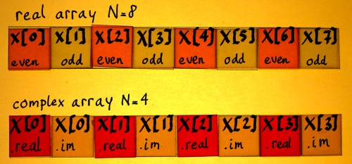
Now is a good moment to introduce the complex datatype, and compare this with the even/odd sequence in a real vector. In C, a complex datatype is nothing more than a struct with two members, real and imaginary variables of type float or double, whatever is normally used for the real vectors.

With the complex datatype, real and imaginary parts are stored in one contiguous array, interleaved in way similar to the sequence of even and odd in a real array. Storing complex numbers in this fashion is both convenient and efficient. Most authors do it this way. I was not so much convinced, until I refactored my FFT routines to datatype complex. They became twice as fast, probably through GNU CC's vector optimizations.

Using the complex datatype, one can no longer feed a real signal in straightaway, like I did on all the preceding pages. But since we are now heading for 'real' FFT, we are going to profit from the new arrangement. A real array can be dereferenced as is, or it can be dereferenced as a complex array of half the length. For this to work, it suffices to declare a pointer of type complex and have it point to the real array, using a regular typecast.

One and the same array can now be dereferenced in two manners:

realarray[n], 0<=n<N

complexarray[n].real and complexarray[n].im, 0<=n<N/2

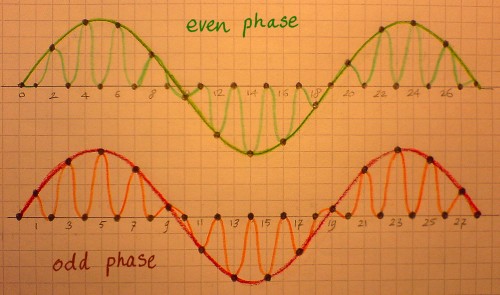
If we process the real array with a complex FFT of framesize N/2, using the complex datatype, the even phase goes into the real input and the odd phase into the imaginary input automatically. Let us have a look at what we are actually feeding in. Here is an example of a cosine with fundamental frequency, and it's even and odd phase drawn as separate half-length vectors:

The even phase represents the original vector downsampled with a factor two. The odd phase is downsampled as well. In addition to that, it has a phase-shift which relates to the one-sample timeshift in the original. What happens when downsampling a signal? All frequencies are doubled, thereby folding negative frequencies precisely over the positive frequencies range and vice versa. So we probably have aliases all over the place. All in all, our task is now much more complicated than extracting spectra of normal input vectors, like it was done on the previous page.

Let us take a closer look at phase decomposition for the moment. Below, I have tried to create an impression of a sinusoid decomposed into even and odd phase. You see the individual phases, not yet downsampled. It is a representation of what each phase contains, if they would exist separately. Because every other sample is set to zero, extra frequencies arise. These are not aliases but images. That is the upsample-counterpart of the aliases. The isolated phases look like upsampled vectors, with all these zeros in them. When we take these zeroed components away and reduce the vectors to half length, the images are gone. But take a close look at the shape of the images: they have opposite sign.

This is a very comfortable phenomenon. It means that aliases, introduced by downsampling the two phases with factor 2, will propagate through the transform in such a way that their spectrum coefficients can later cancel each other. This aspect of phase decomposition is crucial for Fast Fourier Transform in general, and also for Wavelet Transform.

I have plotted an example of such separated but not yet downsampled even and odd phases, fed into real and imaginary input of a normal complex FFT. You see the even phase transformed as real coefficients and the odd phase as imaginary coefficients. The image frequencies, those appearing in the middle of the plot, have opposite signs indeed. This is caused by the one-sample shift of the odd phase, and not by the fact that the odd phase went into the imaginary input.

But we are going to really downsample these phases, take away every other sample and make half-length vectors. These vectors are fed into real and imaginary input of a half-length complex FFT. Of course, this will result in half-length spectra as well. We have to split these spectra, and this can be done using the simple technique that was described on the previous page. I have done an example with split spectra of the same cosine of periodicity 4:

In the even phase's spectrum, the coefficients for the 4th harmonic and it's negative counterpart 28 show up. This is what I would expect: the vector was downsampled, but it was also analysed with a halfsize FFT. For the odd phase, things are less straightforward. It had this one-sample shift, and further it was fed in the imaginary input, so it's spectrum had a rotation over pi/2 radian. This rotation is already compensated in the splitting routine, so you do not see this in the output. What you do see in the output, is the one-sample shift effect.

Maybe you have seen the spectrum plots of Kronecker delta's on my page FFT Output. The plots showed how a one-sample timeshift of a signal effectuates complex multiplication of the spectrum with the fundamental frequency of the transform. This spectral effect can be annulled by complex multiplication in the inverse direction. I have done this on the odd spectrum output, with the following result:

Now we have only real parts left. The negative frequency coefficients in the even and odd phase spectra have opposite sign, as I hoped for. If we now simply add both spectra, we get:

This could be the end result, if you are happy with a 'halfcomplex' spectrum, in which the conjugates are not present. The last actions, complex multiplication off the odd spectrum and summing the spectra, are very similar to a regular twiddle&add/subtract stage in an FFT, only we did not subtract anything because we do not have the negative frequencies part of the output.

I hope that you now feel real FFT is a piece of cake. Below is code for a combined process of splitting even/odd phase spectra and twiddle/add. You could insert code like this after a half-size complex FFT which analysed even/odd phase. Like on the previous page, I leave out the multiplication with 0.5 and do normalisation factor 0.5/N in the forward transform. Pay special attention to the indexing: when casting a real array to type complex, all indexing must be divided by two.

It is funny that all we have done is: splitting spectra, twiddling, and summing spectra again. However there is a big difference in the ways the spectra were merged: in the complex FFT they were summed out of phase, and the last time, where the aliases were killed, they were summed in-phase. Is it now possible to split the in-phase summed spectra again, and go for an inverse FFT? Well, it is normally easier to create aliases than to get rid of them. So I would think that this must be possible. Surprisingly, it can even be done with almost the same operations. We have to twiddle the other way round now, which means flipping the sign of the imaginary twiddle factor. And where we summed the even and odd spectra, we must now subtract. We can re-use the code, with these small adaptations:

Writing the code like this, I wanted to highlight how close it is to the forward version. However the variable names are not precisely to the point anymore, because of the in-phase/out-of-phase difference and the reversed order of operations. You could say that real and imaginary part of the odd phase have swapped their names, anticipating their rotation over pi/2 radians. Below is a version in neutral terms, that can go both ways:

A couple of remarks remain to be made about the halfcomplex spectrum. It does not contain the conjugates, which is generally not really an omission since they do not bear unique information. If needed, we can always compute the conjugates and install the complete spectrum in a bigger array. However if we do not, there is always this nasty Nyquist point to be placed somewhere. The Nyquist frequency bin resides just beyond the half-length complex vector, as it has index N/2. For the sake of compatibility, I have placed the Nyquist coefficient in the imaginary part of index[0], like it is traditionally done.

Since both DC and Nyquist have no imaginary part, they can live together in one complex struct. However, it is a dangerous liason. Imagine you start doing complex multiplications with the spectrum coefficients, while forgetting about the status aparte of bin 0...

For an impression of the format, I plotted the halfcomplex Fourier Transform of a familiar input type. It is clear that the silly appendix on the left should in fact be a real part at the right side of the spectrum, but there was no room for it.

Finally, I have some comments on the normalisation or output magnitude of a halfcomplex spectrum. Because the conjugates are not represented, you see only half of the correlation: the correlation with the positive frequencies. But DC and the Nyquist frequency have no conjugates and I have them fully represented in the halfcomplex spectrum. For spectrum manipulations involving multiplication, this need not be a problem, because such alterations are proportional. But when using the halfcomplex spectrum for analysis purposes, the unique character of the zero bin must be reminded. Of course, one could structurally reduce DC and Nyquist to half it's magnitude in the forward transform and compensate in the inverse, but this could invoke confusion just as well.

For comparison, here is the full complex spectrum of the same Kronecker delta once more: