Norm of Sinusoids

The major feature of sinusoids, making them the jack-of-all-trades amongst waveforms, is their steady, reliable amplitude. On the matrix pages I illustrated how to compute vector norms or amplitudes. These were very small-scale examples with numbers. Now I want to do pictures with curves.

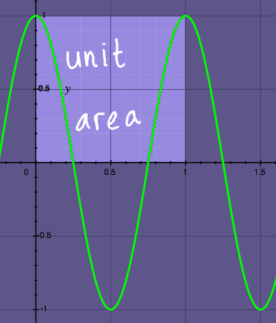
The amplitude of a signal is similar to the integrated absolute (unsigned) area over one period. We are going to find the area of a cosine function with period one, that is, cos(2*pi*x). A unit area of 1x1 is the reference:

How is the area of cosine to be computed? It is clear that if the sample values would be summed, the result over the interval 0-1 would be zero. Half of the samples is negative-valued, and they would exactly cancel the positive values. That is why functions like cosine are defined 'not absolutely integrable'.

We need to find the area in the absolute sense. Like it would be with the cosine function rectified:

At this point, I want to recall the 'Pythagoras-extended' method of computing a vector norm or amplitude. Functions like cosine are called 'square-integrable' functions. The method for computing their area is very similar to computing a vector norm in the discrete case:

To compute the amplitude of a sampled cosine function with period one would require these steps:

- square all it's sampled values over the interval of one period
- sum the squares; this gives the inner product, the total energy
- divide this sum by the number of samples: this gives the energy
  independently of the number of samples, as a portion or fraction of 1
- take the square root of the energy value: that gives the amplitude

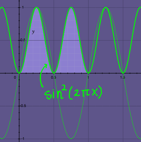
These steps can be visualized to a certain extent. Below, we see the cosine function squared. The area under the squared cosine covers half a unit area.

The inner product, or energy, or norm-squared, of cosine is 0.5. To compute the norm or amplitude is now simple: take the square root of 0.5. It is around 0.707. The norm of a cosine function over a full period is 0.707, or more precise, the square root of 0.5.

Below is the figure for sin(2*pi*x) and the square of it. Not surprisingly, sine has the same amplitude as cosine: 0.707, or more precisely the square root of 0.5.

I want to know what will happen when the peak-value of cosine is reduced from 1 to 0.5. So I plot 0.5(cos(2*pi*x) and the square of that. Inspecting the area under the squared curve, I guess it is 0.125. That is the energy, and the amplitude should be the root of this: 0.3535. Hey, that is exactly half of 0.707.

Drawing conclusions from one example is dangerous. Here is another example with 0.8cos(2*pi*x), and the squared curve peaking to 0.64. The area under the squared curve is 0.32 and the root of that is around 0.566. That must be the amplitude of 0.8*cos. And indeed, 0.8*0.707 is 0.5656.

Although the peak value of cosine is not it's amplitude, a variation in the peak value is proportional to a variation in the amplitude. That is handy.

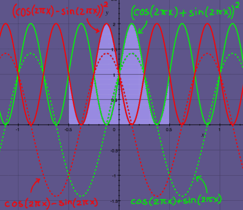
Now I am curious, what will happen when sine and cosine are summed? I will plot the sum, and the square of the sum. The area of the squared sum signal seems to be exactly 1. The combination has unit energy. And because the square of 1 is 1, it has unit amplitude as well. From the picture, the peak-to-peak value of the sum signal can also be estimated. It is around 1.4. The precise value would be the square root of two.

Sine and cosine have steady amplitudes. Their combined amplitude is unity amplitude over the interval [0,1]. But it is also unity when you look at it pointwise, sample by sample. From the sinusoidal curves it is impossible to see this at a glance. Therefore I have drawn a couple of example points on the curves, and their corresponding complex exponentials on the unit circle:

Speaking of complex vectors, what about their conjugates, with the negative imaginary parts? I plotted the summed conjugate vectors with period one, and their squares. Considering the symmetry of the conjugates, it would be natural to integrate over a unit interval centered round zero, so [-0.5, 0.5]. Again, the total area covered is unity, and so would be the area of the square root.

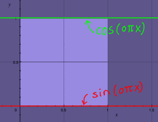
There is a couple of special cases for sinusoid amplitudes. The first one is that of cos(0x) and sin(0x). Their 'curves' are shown below; they are perfectly straight lines at y=1 and y=0 respectively. These are functions with infinite period. So strictly speaking, they are not integrable, not even square integrable. Still, it can be argumented that the amplitude of cos(0x) over a unit interval is 1. And the amplitude of sin(0x) over a unit interval is zero. The plot below illustrates this case. In engineering terminology it is known as the direct current or DC case.

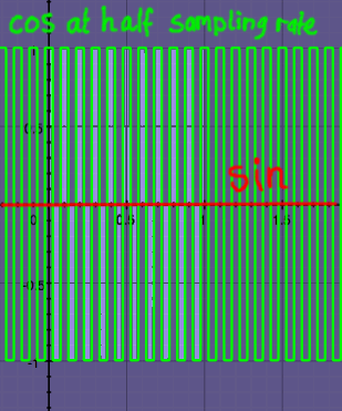
The second special case of sinusoid amplitude does not look sinusoidal either. It is the case of discrete sinusoids at half the sampling rate of a system. A cosine looks like a square wave under this condition, because it alternates from peak to peak without inbetween values. As a square wave, it has amplitude 1. A sine wave can not exist at half the sampling rate, because it's peaks would fall precisely in between the sample points. So it has amplitude zero by definition.

The mathematical interpretation of these special cases is: they are pure real functions, and have no conjugates. They can not have that, because there is no imaginary part. Or, you could say, they are their own conjugates. So, a unity DC component could be expressed:

In a matrix with complex conjugate vectors, DC and the half-sampling-rate vectors are represented with only one vector each.

Much more can be said about sinusoid integrals. On this page, I have summed sine and cosine, and their combined amplitude is unity. On the next page, I will multiply sine and cosine. That will show yet another useful surprise.