
While the page FFT Window and Overlap
illustrated some minute details of windowing in general, I now want to
find the best windowing strategy for spectral filtering. My parametric
Fourier filter routine has the following basic filter spectrum curve:
|
A logarithmic sweep, clipped at the top, with variable width and
position. When shifted over the frequencies range, the bandwidth is
adjusted automatically so the Q factor is retained.
In a log sweep the left side slope is always the steepest, and it
gets steeper automatically when the curve is shifted towards the lower
frequencies. Steep flanks in a filter
spectrum can cause us troubles, and since I want to push it to the
limit, I need to know where the limit is and what it looks like.
Allegedly, brickwall filtering exceeds the limit of what can be
done. I have learned that at school, but I could never imagine what the
precise effect is. Therefore I will now perform some simple
spectrum-mutilation experiments and
see what
happens.
Below is a test function plotted. It is a windowed cosine of
periodicity 3. A modulated window function, one could say as well.
 |
The spectrum coefficients of the modulated Hann-window are:
X[2] = 0.125
X[3] = 0.25
X[4] = 0.125
and their conjugates
Mutilating the wave's spectrum with surgical precision, I will now
remove the X[4]
coefficient and it's conjugate from the spectrum, and revert to time
domain:
 |
Oops. Seeing the plot, it is hard to imagine that I could not
imagine this. The window is partly undone. That is how I perceive it,
because I would like to filter any frequency but not the window. But this is only
one way to perceive the effect. Let us think a little longer about it.
In fact, the original coefficients represented:
0.25 * cos((2*pi*x/N)*2) second harmonic
0.5 * cos((2*pi*x/N)*3) third harmonic
0.25 * cos((2*pi*x/N)*4) fourth harmonic
The third harmonic I consider the test input frequency, and the
second and fourth harmonic are the sum and difference frequencies
resulting from multiplication with the window. The combination appears
as a windowed function within the FFT frame. Successive frames look
like this:
 |
With coefficient X[4] removed, the reconstruction is still periodic
without discontinuities, and contains two frequencies of unequal
amplitude:
 |
But these are not the signals that we are going to hear. I have to
find the result of overlapping frames. With two times overlap, each
successive frame is time-shifted by N/2. The window function remains
centered in the frame, but the input functions are phase-shifted, and
for a cosines of
periodicity 1 and 3 this happens to be a sign-inversion. The sum of
overlapping frames, each still having all three harmonics, is exactly
that single harmonic 3:
 |
And here is the sum of overlapping frames where the X[4] coefficient
was taken out:
 |
Amazing! The original input is still restored. This must be sheer
coincidence, or not? Was my example too simplistic to reveal the
downside effects?
Yes, the example input frequency harmonised with the framesize, so
it is an exceptional
case. Still it shows a mechanism that is also at work for non-harmonic
frequencies. To understand what is happening here, we must
temporarily
adopt another perspective on windowing and overlap. The window is to be
perceived as a set of two (or more) functions. One is the DC component,
and it's task is to preserve the original signal with a certain
magnitude factor, like 0.5. The other function is a modulator,
converting the original input frequencies into sum- and difference
frequencies, also with a magnitude around 0.5. In the Hann window, and
some others, the modulator is just the FFT's fundamental cosine. That
is an uneven frequency, and from this comes the special effect in
overlapping FFT frames. Every half period, it's sign is flipped. So in
overlapping frames, though the window is always the same, it's cosine
component is
everytime flipped respective to the analysed signal. I hope the
following figure can make this clear:
 |
Notice that the window's DC component does not flip sign. Therefore,
the original frequencies are analysed and restored as they are, with
amplitude factor 0.5 + 0.5 = 1 for the overlapping frames. The sum- and
difference frequencies however, as generated by the signflipping cosine
component, have different sign for the even and uneven numbered FFT
frames. They cancel themselves in the sum signal as it is
reconstructed. The fattened main lobes in a spectrum are partly built
of antimatter!
Now I want to try a test wave inharmonic with the FFT size:
periodicity 10.2. I picked coefficient 11 (and it's conjugate) off the
spectrum. To my surprise, the wave came out untouched. But then I
zeroed coefficient 10. This really spoilt the wave. While it fades, it
is heavily distorted, and be shure that it sounds rotten (that is, if
you want things neatly processed). The visible kink produces a high
frequency rattle, but there is also a low frequency product in the
sound,
possibly originating from the overlapping FFT periodicity.
 |
So - does the antimatter trick no longer work here? The case of an
input frequency inharmonic with the FFT size is much more complicated.
The discontinuities at the frame borders begin to play their role.
Although a Hann window looks smooth, it is actually a sum of two
functions which are both not smooth at all. The DC component in a
window is an attenuated rectangle window, and the cosine term is
chopped as well.
 |
These chop cuts are responsible for extra frequencies, which we can
see if the chopped functions are analysed within a wider frame, padded
with a lot of zero's on the left and right. The previous page showed Dirichlet kernels
representing spectra of chopped functions. Time-shifting the chopped
fundamental cosine by N/2 will sign-flip it's Dirichletish spectrum.
This part of the window retains it's function, no matter if the input
frequency harmonizes with the FFT size or not. It is the rectangular
part of the window that causes us troubles. This part was intended to
act as an identity, preserving the input frequency. But now it turns
out that this window part produces sum- and difference frequencies as
well. And, since the rectangular part does not phase-shift over time,
these products do not annihilate themselves in the reconstruction with
overlapping frames. If we take out coefficient 10, the input frequency
is attenuated, but the products caused by the rectangular part of the
window will survive. In the spectrum, these products were phase-hidden
by the cosine window products, but in the overlapping reconstruction
they are neatly restored. What you see is not what you get! For
such a case, the output result is very similar to
non-windowed processing.
Using a Hann window, I have checked that a gradual attenuation in
the
spectrum, running over three coefficients, worked without
generating audible artefacts:
x[9] = 1.00
x[10] = 0.75
x[11] = 0.50
x[12] = 0.25
x[13] = 0.00
x[14] = 0.00 etc
In my Fourier filter with it's extreme filter options, spectrum
flanks much steeper than this can happen. Is there any window type that
can handle such abuse? Using the
Max Msp pfft~/fftin~/fftout~ objects, I definitely have smoother sound
from the same Fourier filter process, than with my own C code.
 |
the resynthesis window: brickwall me
Admittedly, I have been puzzled by this matter for more than a week,
while the answer is soooo simple. It is embarrasing. I have been using
the window before analysis
all the time, while it is much more important to have one after resynthesis. Shall I now
rewrite this whole page, and never mention how I bungled around with an
analysis window? Hmmmm... the analysis experiments revealed some
effects that must be at work in a resynthesis window as well, and I
still want to understand why and how things work.
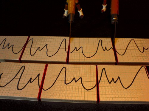
Let me first state that hard cut brickwalling with very low artefact
level is possible, if only you use enough FFT overlap, and windows
before and after transform. The wacky scope trace below can not be
proof of
that, but believe me, it sounds a hundred times better than before.
 |
Is there a way to visualise what is actually happening? Let me
produce a very simplistic testcase: a cosine input of periodicity 1.5
respective to the FFT framesize, as inharmonic as can be. I do not
window this cosine before analysis. In it's spectrum, I eliminate
coefficients 1, 2, and their conjugates N-1 and N-2. After IFFT, there
is still quite a lot of output, as the figure on the right below shows:
 |
 |
The mutilated wave still has the periodicity of the input, but the
frequency content is completely altered. At the frame borders, it has a
spiky shape. The output largely represents the difference between a
cosine of infinite length and a chopped cosine. So it represents the
cuts, respective to the cosine that I had tried to remove. Like a
deflated balloon, glued to the frame edges. Rather alarming, how much
signal energy there is still left.
But now I am going to window this output signal:
 |
There. The most offending element is already gone. But what will
happen to the remainder? That is harder to grasp.
When we windowed the input signal, the overlapping frames were
time-shifted snapshots of one and the same signal stream everytime.
Therefore, the sum- and difference frequencies resulting from the
window-modulation, propagating through the transforms, were perfectly
undone in the overlapping reconstruction of the signal. In contrast,
the transform artefacts were not modulated, only summed to the total
output.
The even- and odd-numbered IFFT output frames however (assuming two
times FFT overlap here) do not represent one and the same signal. The
original input components coincide, but eventual transform artefacts
pop up
alternating. If we window each IFFT output frame and then sum the
frames, the overlap will not by definition undo all modulation
products. The elimination of boundary spikes is the most conspicuous
aspect of this mechanism. Theoretically, every new frequency component
that was generated as a
side-effect of the frame-by-frame processing, is a candidate for
elimination. The artefacts are however not identical in successive
frames, so their elimination is not guaranteed. The more overlap, the
better elimination.
 |
To summarize the decisive difference between analysis and
resynthesis window: while the analysis window temporarily repositions
the frame boundary effects, the resynthesis window boldly eliminates
them in the output. It is best to use them both, but the resynthesis
window does most of the work. By the way, using two windows in series
means that they are actually squared. Therefore, you need at least four
times FFT overlap to produce a constant window sum.
At last. I can now test some window types in practice.
I compared Hann and Blackman, feeding a pure sinusoid of variable
frequency through a 1024 point spectral filter that zeroes everything
below or above a chosen brick wall cut off point. Starting out with
four times FFT overlap, both window types seem to produce a similar
type of artefact: around the cut off point, where the input fades, a
faint undertone is produced. With the Hann window, it is very hard to
perceive this tone, but with Blackman it's level is higher.
Scaling up to eight times overlap, I can no longer hear any
product frequency. There is only a smooth fade out of the input
frequency. The window type does not matter. Hann and
Blackman do this job equally well.
Now that brickwall filtering seems to be a realistic option, I
want to know the specifications of the output. What is the filter
slope? I checked the dB output for a 1024 point lo pass filter with a
hard cut off between FFT bin 10 and 11. Here are the attenuation values
for the center frequencies of some bins:
bin 10: - 1.5 dB
bin 11: - 13.5 dB
bin 12: - 45.5 dB
bin 13: - 93 dB
Inbetween these values,
the decay is smooth. This was with Blackman windows. Using Hann
windows, the -93 dB point was already at bin 12, so the slope is
actually steeper than with Blackman. I repeated those measurements at
other frequencies, resulting in equivalent bin attenuation
values. So, in the output, the slope is not a brickwall. It is probably
sinusoidal, albeit extremely narrow. The above mentioned values are for
8 times overlap. With 4 times overlap, the decay in the first bins is
equivalent, but further away there seem to be higher ripples than with
8 times overlap.
The measurements made me realise that specifications of brickwall
filtering in frequency domain can not be expressed in dB per octave.
Neither can it be expressed
in dB per bin, since that has a non-linear relation. But you could
define it
in terms of decay over the first bin interval or decay over the first
two bin intervals. And a bin interval is a single-harmonic interval.
What that means in Herz depends on FFT framesize, sampling rate, and
position within the spectrum. At the low end of the spectrum, the bin 1
- 2 interval is one octave indeed. (The bin 0 - 1 interval is undefined
in terms of octaves, it is infinitely many octaves). The bin 1 - 4
interval is two octaves, and you can easily produce -93 dB attenuation
over that interval. At all higher positions in the spectrum, the figure
is (much) better.
The one thing that you can not do with spectral filtering, is to
selectively eliminate or attenuate a frequency within a bin. Because, there really
is only one frequency defined per bin. In the low frequencies range,
that can certainly be an issue. But the virtue of a brickwall-proof
filter setup is, that at least the sound can not be spoilt by an
attempt
to push things to the limit.
conclusion
After these experiments, my personal windowing preference for
spectral processing would be: four times overlap, using Hann windows
before analysis and after resynthesis. The artefact level is so low,
that it can not really be perceived otherwise than in test conditions.
The Blackman window leaves louder modulation frequencies, possibly
because of it's second harmonic cosine component which has less optimal
sign-flipping behaviour in overlapping frames.
I am now getting used to four times overlap as the minimum for FFT
processing. It is not even so computationally intensive. On my 2
GHz MacBook, the complete filter process is responsible for slightly
over 1 %
cpu load in realtime at 44k1 sampling rate.