
exponentials
Complex exponentials are extremely useful in frequency analysis and
in computing complex coefficients according to (user) parameters on
frequency.
From their name you would guess that it must be like: complex numbers
in the exponent of some base. As if complex numbers are not yet complex
enough. It may be useful to review ordinary exponentials first
and then extend to complex exponentials.
|
Aha. Not surprising. It is too difficult for them. They are good
with circles and straight lines.
Think of this: complex exponentials
were invented in the 18th century. How could
mathematicians generate a multitude of datapoints for that type of
functions? Actually, exponentials and their
counterparts logarithms were very popular at the time, and voluminous
data tables (also for trigonometrics) were available.
Still, I am happy
to go the easy way with Grapher. Here is a couple of real exponential
functions on different bases:
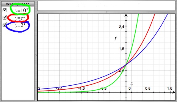 |
The variable x is in the exponent, and the constant is called the
base. A typical point that all
exponential functions share, is at x=0 where y is 1. Any number to the
power of zero is defined 1.
One of the functions in the graph has base e.
A letter again, after i and pi. Of all possible bases, this is the
indicated one for complex exponentials, although the compelling reason
for that cannot be expressed in a few words. The number e is an important
mathematical
constant, with value 2.71828 (and infinitely more decimals).
Before going to complex exponentials, let us recall what is so
useful about exponentials. When multiplying powers of the same base,
the exponents can be added, like in:
 |
 |
I know, I know.... the example seems trivial. But it has its use.
Look, this is a complex exponential:
 |
It has the complex number (0+i1) or simply (0+i) in the exponent of
e. As the real part is zero, the complex number is even a pure
imaginary number. And then I chose the simplest of imaginaries, the imaginary unit, for this example.
Remember, the real part and the imaginary part within a complex
vector are not to be summed, because they belong to different
directions. Now it turns out that splitting can be as convenient as
merging:
 |
We then have a real exponential and an imaginary exponential as
factors.
The real exponential could be computed as a number, which in this case
is 1. Therefore it reduces to:
 |
That looks simple enough, but whtthfck does it mean??? It is hard to
derive the meaning of such a number from what we know about the
non-exponential complex numbers.
You may rightfully expect that successive powers of a complex number
will show
a rotation-like pattern, like complex multiplication does in general.
Of course, there are infinitely many complex powers of e conceivable,
not only the integer powers. And wait, what about that factor e0 that we have so
neatly written out of the complex exponential? It is the real number 1.
Sounds like the unit circle?
 |
It starts on the real axis of the complex plane, with
 |
But soon as the slightest imaginary part come into the exponentials,
they start their circular pattern. The real exponential e0
as a steady factor stands for a radius of length 1. So here is the unit
circle indeed.
Still all the above does not clarify the positions of complex
exponentials on the complex plane. What is the pattern? It is found in:
 |
This relation was stated and proven in the 18th century by Leonhardt
Euler. He demonstrated how the combined Taylor series expansions of
sine
and cosine functions coincide exactly with the Taylor series of
exponents on e.
Although the details of the mathematical proof are interesting and
not too complicated, I would rather like to skip that. Instead, I let
Grapher show what will happen if a base other than e is chosen for a complex
exponential. The plot is on the real plane where circles of the complex
plane appear as sinusoids:
 |
A complex exponential function on base e appears to be the one that relates 2pi to a full period. Other bases would result in circles as well, but they would go too fast or too slow to have their imaginary exponent exactly expressing radians.
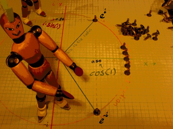
We can recycle the drawing with 1-radian angles on the unit
circle that was used on the previous page, and place ei and e-i
to illustrate the relation of angles and imaginary exponentials:
 |
And in the other quadrants:
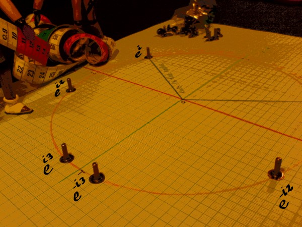 |
Each integer-imaginary-power of e
points to a multiple of one radian.
Other frequently referenced points are:
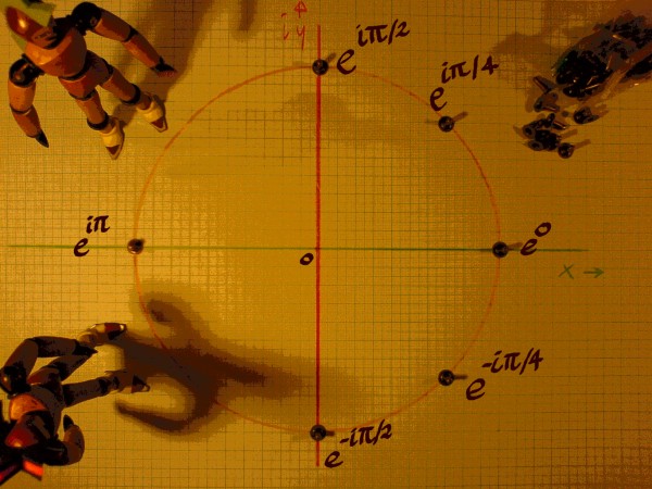 |
Now we know where to position pure imaginary exponentials. They are
called 'unit vectors' because they have radius length 1. As such, they
represent a pure rotation. Multiplying a complex number by a unit
vector will not alter the radius of that complex number.
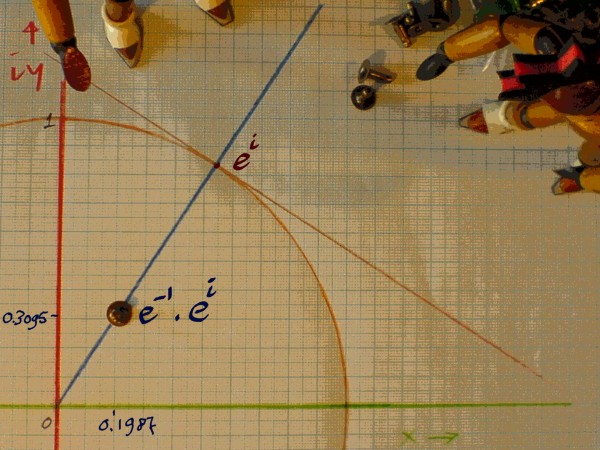
But where must the real part of a complex exponential reside? Till here I have worked with the comfortable value e0, but what if it is different? Look, if you draw a tangent on the unit circle, here for the example of e-1+i, the radius or amplitude line clearly shows up as an axis perpendicular to the unit circle. The real factor in the complex exponential is the amplitude, or radius. In the example it is e-1 and that is about 0.3678.
 |
Let us now calculate the complex number (x+iy) for e-1+i,
and check whether the result supports the statements I have made on
this page:
|
e-1+i = |
 |
Arithmetics seem to be in accordance with geometry in this case.
Of course, some applications ask for the inverse route: transform
a complex number (x+iy) to a complex exponential form e(a+iß).
The following steps
are required:
Summarized: (x+iy)=e(ln(sqrt(x^2+y^2))+i(atan(y,x)). To
this I have two comments. Very often, the radius is not
transformed to a real exponential even when the angle is expressed as
an
imaginary exponential. Then it reads like: r*eiß,
where r
stands for radius. This form may be just as convenient in mathematical
operations.
The other thing is: to
find an angle from a complex number you will soon need an arctangent
function
that takes two arguments, y and x respectively. It is in the standard C
library so math and dsp software may offer the function. The arctangent
function
for a single argument (y/x), found in many pocket calculators, is
restricted to angles from -pi/2 to pi/2.