Fourier Matrix

Imagine you have a signal and you want to examine how much of a certain frequency is in that signal. That could be done with two convolutions. The signal would be convolved with the two orthogonal phases, sine and cosine, of the frequency under examination. At every samplemoment two inner products will tell the (not yet normalised) correlation over the past N samples. Below, I plotted an example of sine and cosine vectors doing one cycle in N = 8 samples:

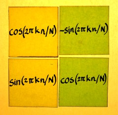
Recall that convolution vectors always appear time-reversed in the convolution matrix. To time-reverse a sine-cosine set we do not need to inspect the signal sample by sample to flip the array. Take a look at the plot below, and the next one. A set of cosine and negative sine has exactly the same property as a time-reversed set.

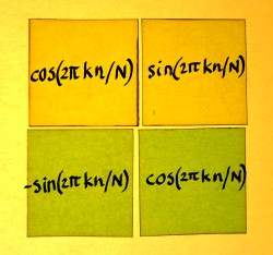
In complex number terminology, it is the complex conjugate. cos(x)+isin(x) becomes cos(x)-isin(x):

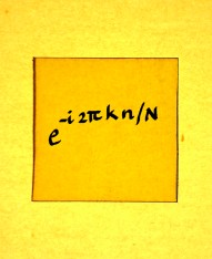
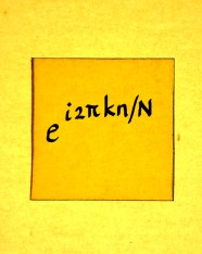
These vectors can be described as an array of complex numbers cos(2*pi*n/8)-isin(2*pi*n/8) or as complex exponentials e^-i2*pi*n/8. The complex numbers or exponentials are on the unit circle in the complex plane, with the series showing a negative (=clockwise, yes) rotation:

To compute these convolutions would require 2 times 8 multiplications, is 16 multiplications per samplemoment, and almost as many additions. Now imagine you would like to detect more frequencies than only this one. For lower frequencies the arrays must be longer. At a typical samplerate of 44.1 KHz, one period of 40Hz stretches over more than a thousand samples.

Computing convolutions with thousand-or-more-point arrays, just to find a frequency in a signal, would be a ludicrous waste of computational effort. After all, the amplitude in a complex sinusoid vector is perfectly constant. Therefore it would almost suffice to take a snapshot of the signal every N moments, and compute the inner product once over that period. This will come at the price of probable jumps at the boundaries of the snapshot. Such jumps form artefacts which will distort the correlation. So the snapshot method is a compromise. But a necessary one, specially since you may want to detect more frequencies, covering the whole spectrum.

Convolution with 'snapshots' is not convolution in the proper sense. Though it can be filed under 'block-convolution'. With block-convolution, we could resolve up to N frequencies (conjugates or aliases included) in each N-point snapshot. The block of a Discrete Fourier Transform is an NxN square matrix with complex entries. The blocks themselves are positioned on the main diagonal of a bigger matrix. We will take a look at that from a bird's-eye-perspective:

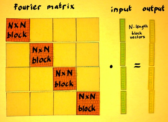Compared to regular convolution, a big difference is: the shift in the rows of the Fourier matrix. It shifts rightwards with N samples at a time instead of one sample at a time. It also shifts downwards with N samples at a time. The output is therefore no longer one signal, but N interleaved points of N separate  N-times downsampled signals. Which were filtered by the N different vectors in the Fourier block.

This is not a conventional interpretation of Discrete Fourier Transform. But I do not worry about that. There is enough conventional descriptions of Fourier Transform in textbooks and on the web.

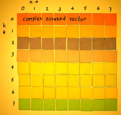
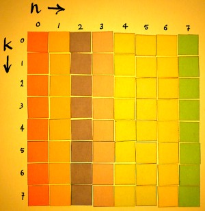
Let us now find out how to fill a Fourier block. Our example is with N=8. We need to construct 8 complex vectors of different (orthogonal) frequencies. Because I have the habit of indexing signals with n, like x[n], I will reserve index k for the frequencies. The frequencies go in the rows of the matrix.

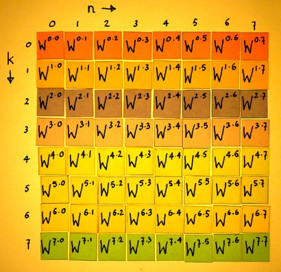
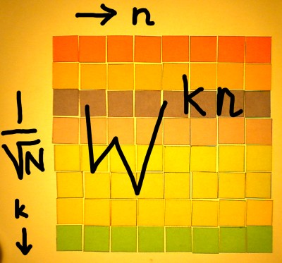
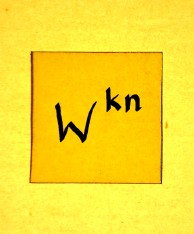
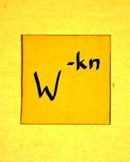
All entries will be filled with complex exponentials e^-i2*pi*k*n/N. For convenience, we write e^-i2*pi*k*n/N = W^k*n. Then, the Fourier matrix can be simply denoted: the W^k*n matrix. No matter how big it is. There is always just as many frequencies k as there are sample values n.

In this definition, W can be recognised as a complex number constant, defined by the value of N. The number N divides the unit circle in N equal portions. W is the first point in clockwise direction, thereby establishing the basic angular interval of the matrix.

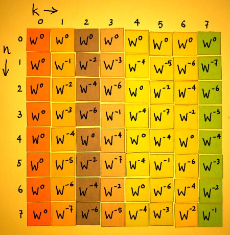
In the figure below, the matrix is filled with the W^kn powers:

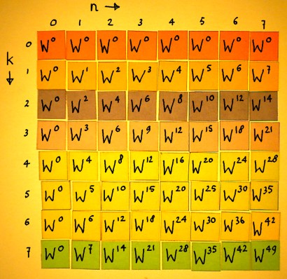
Do the multiplications:

Row number k=0 represents DC, with e^-i2*pi*k*n/N being e⁰ⁱ in every entry. Row number k=1 represents the fundamental frequency of the matrix, doing one cycle in 8 samples. This is the complex vector that I took as the first example earlier on this page. Row number k=2 represents a frequency going twice as fast. It is the second harmonic. Here is a plot of sine and cosine in the second harmonic:

The third harmonic does three cycles in 8 samples:

Everytime, complex exponentials of the fundamental period are recycled. No new exponentials will appear. Here is how the third harmonic moves round the unit circle on the complex plane:

The next one is the fourth harmonic. In the case of N=8, the fourth harmonic is the famous Nyquist-frequency. Sine cannot exist here. On the complex plane, the only points are -1 and 1 on the x-axis.

The fifth harmonic is the mirror-symmetric version of the third harmonic.

When their iterations over the unit circle are compared, their kinship is clear:

They are conjugates. To put it in other words: if the third harmonic would rotate in reversed direction, it would be identical to the fifth harmonic. But all harmonics have a well-defined rotational direction, because they are complex. All vectors are unique, and orthogonal to each other. Such conjugate distinction, by the way, can not exist in a real (input) signal: there we speak of aliases.

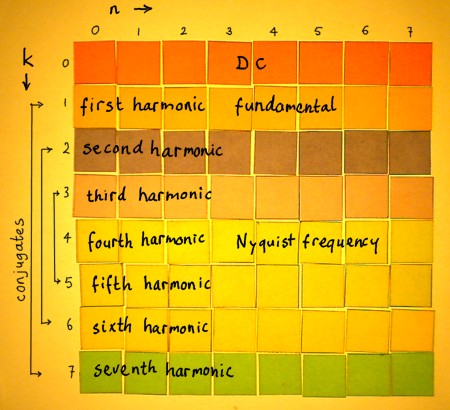
The sixth and seventh harmonic are also conjugates of other harmonics in the matrix. When an overview of the harmonics is made, it becomes clear that row k=0 and row k=4 have no conjugates. These are DC and Nyquist-frequency.

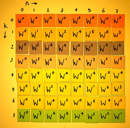
Because the powers W^kn are periodic modulo N, the vectors can be rewritten. W⁸ is equal to W⁰, W⁹ is W¹ etcetera. It is integer division by 8, and the remainder is the new exponent of W. In the rewritten Fourier matrix for N=8, the conjugates display themselves quite clearly:

We are not completely done with the Fourier matrix yet, because it needs normalisation. There is a certain freedom, to choose a normalisation type according to the purpose of the transform. I have done a separate page on that because it is too complicated to describe in just a few words. But strictly speaking, a normalised vector is a vector with norm 1, or unity total amplitude. That requires a normalisation factor 1/N^1/2 for all entries of the W^kn matrix. In that case, the Fourier matrix is orthonormal, and the transpose of it is exactly the inverse. An orthonormal Fourier matrix can be defined:

The output of the matrix operation is called 'spectrum'. It expresses the input content in terms of the trigonometric functions of the Fourier matrix. These functions are pure rotations, and the output coefficients tell the amount of each, as found in the input. The normalisation type is crucial to the interpretation of these coefficients. And the transform block-width N is decisive for the frequency resolution.

Apart from being informative about frequencies, the coefficients have other virtues. They can be exploited to manipulate the frequency content. After such manipulation, the inverse Fourier Transform can revert the spectrum back to where it came from: time, space, or whatever the input represented.

To construct the inverse Fourier matrix, we have to find the transpose. Normally, that can be done by turning the rows into columns. So it would look something like this:

But I have not yet written the entries, because there is something special with these. They are complex, and need to be transposed as well. This is a good moment to inspect the complex entries in detail. On the matrix pages I described complex multiplication more than once. It has a 2x2 square matrix. Therefore, one complex W^kn entry is actually four real entries:

When the rows of the 2x2 matrix become the columns, we simply get the complex conjugate. The complex exponential then rotates anti-clockwise, which is called positive. The sign in the exponent of W^kn must flip and it becomes W^-kn.

Now I can write the W^kn powers in the entries of the transpose:

The only difference with the original matrix is the direction of rotation. Apart from their sign, the powers of W have not changed. The matrix is almost symmetric over it's diagonal. The only thing that is not symmetric, is hidden within the 2x2 complex matrices behind the W^kn entries.

The normalised Fourier matrix and it's inverse can be visualised:

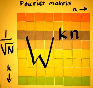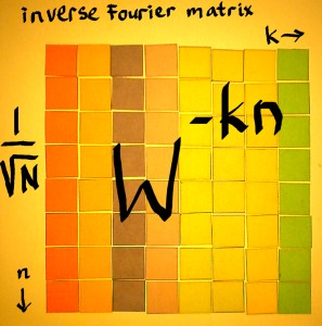It can be written algebraically, with the hatted x being the transformed array:

And the inverse transform:

Discrete Fourier Transform is a very clear and systematic operation, therefore the description of it can be so concise. But the formula is only the principle of DFT. Implementation of the transform will require adaptations, in order to reduce the amount of computations in one way or another. For the transform of a real signal with small block-width N, computation of the conjugates can be skipped. For large N, factorisation of the complex matrix makes for efficient algorithms. Then we speak of the Fast Fourier Transform. Whish I could sketch an FFT operation with my coloured square paperlets....