Step Two FFT

The previous page showed how a Fourier matrix can be decomposed into sparse factors, making for Fast Fourier Transform. The factor matrices multiplied showed a Fourier Matrix with it's spectrum decimated. For the purpose of that demonstration, the factor matrices were not yet optimally decomposed. On this page we go one step further. Well actually we will go back to our roots once more, the roots of unity.

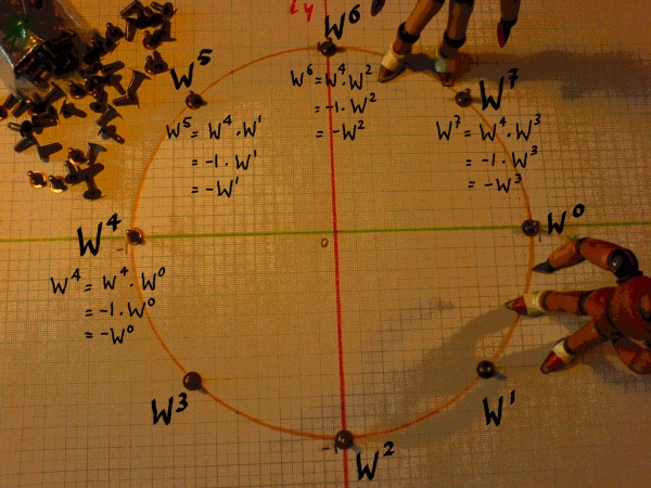
We will make use of this 'identity':

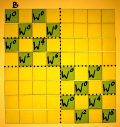
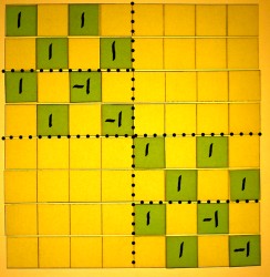
In our N=8 example FFT, W^N/2 is W⁴. For other N it would not be W⁴ of course. Anyway, -1 is the primitive square root of unity. With the help of this we are going to find aliases that will enable a further reduction in the amount of computations. In the picture below, aliases for W⁴ till W⁷ are written down.

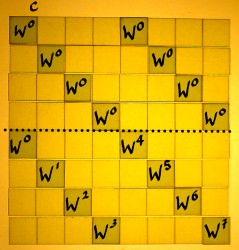
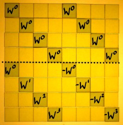
The eight-powers of unity in our FFT matrix are rewritten in this fashion. On the left is the original matrix, the translated version is on the right:

Translating the next factor matrix:

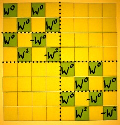And the last one:

So what is our gain here? Normally, you first multiply corresponding cells in vectors and then sum the results to find the inner product. In the radix 2 FFT there is two non-zero entries per row. That would mean two multiplications every time, followed by an addition. But in the case that two multiplication factors were the same, you could first do the addition and then the multiplication. In the above case, the factors are not equal, but almost: only their sign is different. Then it would suffice to first subtract and subsequently multiply. That saves one complex multiplication. Compare with a real number example like: 4*5-2*5=(4-2)*5.

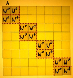
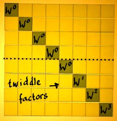
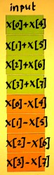
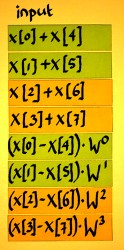
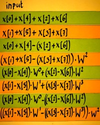
Let me split the first FFT factor into an addition/subtraction part and a rotation part. The rotation matrix has what they call the 'twiddle factors'. The addition/subtraction part comes first, because we work from right to left.

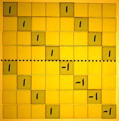
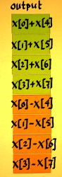
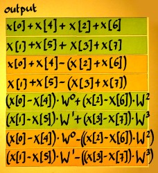
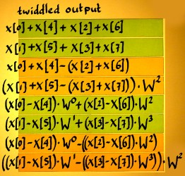
Below, the output of the first matrix operation is illustrated. Subtraction is computationally no more intensive than addition. But in the process, the entries x[4], x[5], x[6] and x[7] get a 'free' rotation by pi radians or half a cycle.

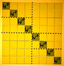
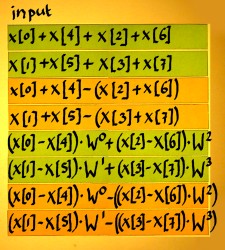
Next comes the multiplication with twiddle factors:

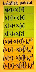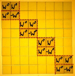
The two remaining FFT stages are decomposed similarly, into an addition/subtraction matrix and a diagonal rotation or 'twiddle' matrix. I will draw these decompositions as well. Here is the second stage as decomposed in addition/subtraction and twiddle matrix:

First do the additions and subtractions. Notice how input and output vectors are treated here as if they were two-point vectors, while in the preceding stage they were four-point vectors.

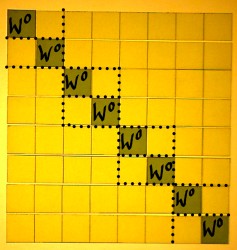
Next comes the twiddle matrix of the second stage:

In the third stage, the twiddle matrix has merely W⁰ factors. This will function as an identity matrix so we do not have to implement it. Only the matrix with additions and subtractions remains to be done.

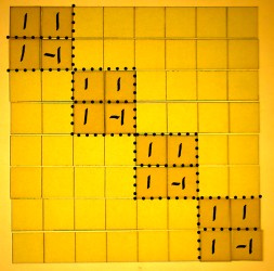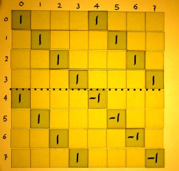
The last operation is thus addition and subtraction:

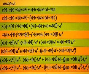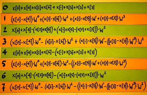
Below, I reorganised the output bins to bitreversed sequence, to have them in their harmonic order. Now you could check if the FFT tricks have worked. Bin number 4 for example, has the even x[n] with positive sign and the odd x[n] with negative sign. This is equivalent to x[0]*W⁰, x[1]*W⁴, x[2]*W⁰, x[3]*W⁴ etcetera.

The other harmonics require more effort to recognize them as being complex power series. But they all are, it is just that they are computed via another route.