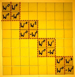
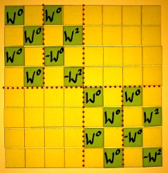
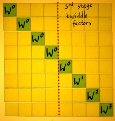
Even when we confine ourselves to radix 2 FFT, there are four basic schemes. They are the classic Cooley-Tukey and Sande-Tukey algorithms. Only one of these was illustrated on the preceding pages. I want to explore the other three schemes as well. They have so much in common, yet the differences are decisive and they are not to be mixed or confused. First I will discuss some details of these differences. At the end of this page, the four schemes are put together, for overview. They are matrix visualisations of butterfly graphs like those printed in The Fast Fourier Transform (p. 181) by E. Orhan Brigham.
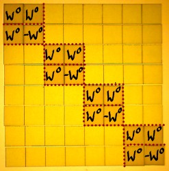
For comparison, here is the scheme as it was illustrated on the
previous page:
|
|
|
|
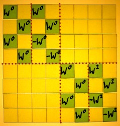
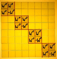
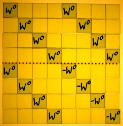
The second scheme differs from the first one in the sense that it
starts with the square roots of unity, instead of ending with them.
Recall that we work from right to left. Further, the identity parts and
rotation parts are now left/right organised, instead of top/bottom. The
output of this scheme would have a decimated spectrum as well.
 |
 |
 |
|
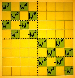
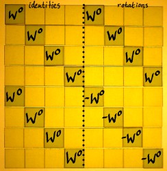
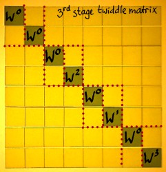
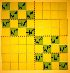
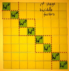
Using this scheme, the twiddle matrix would precede the additions
and subtractions, in every stage. As an example I will decompose the
third stage:
 |
 |
 |
The twiddle factors do not appear in their natural order. From my
small example it is hard to see the pattern of it, as we only see W2,
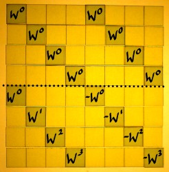
W1 and W3. If the third stage is depicted in it's
non-optimized form, it becomes clearer.
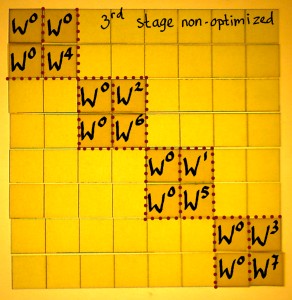 |
On the left I have written all rotations as positive powers of
W. The series is:
This is a pattern we have seen before. It is bit-reversed. Of
course, this will have a different meaning in every stage of the FFT.
The 8th roots of unity have three bits, the 4th roots have two bits,
and the square roots have one bit. |
So in this scheme we have to apply the twiddle factors in
bit-reversed order, and the output is also in bit-reversed order. Then
the question arises if the twiddle factors can be used in their natural
order, to have the output in natural order as well. I have tried that,
just for curiosity. If it would work, everyone would use that of
course. But it does not work. Decimation is the essence of FFT. Recall
that downsampling is also a form of rotation. It doubles a frequency
everytime. As such it is part of the strategy for getting all rotation
factors at their proper position. Without it, output bin number 1 for
example would have these nonsense values:
x[0]+x[4]+x[2]+x[6] + (x[1]+x[5]+x[3]+x[7])*W1
Downsampling W1 gives W2, and downsampling one more time gives W4. Then it makes sense, being the correlation output of harmonic number 4.
x[0]+x[4]+x[2]+x[6] + (x[1]+x[5]+x[3]+x[7])*W4
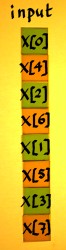
Decimation brings us to subsequent schemes, in which the input
signal is reorganised with indexes bit-reversed, before all other
operations. The output will
appear with the frequencies in natural order.
 |
 |
 |
 |
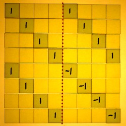
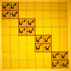
This scheme has 'first-twiddle-then-add&subtract'. As an
example, I sketch the third FFT stage here below, because in the other
ones there is less to see. The twiddle factors appear in their natural
order.
 |
 |
|
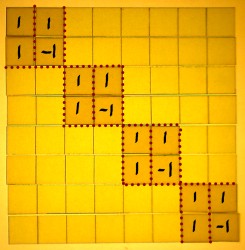
There is one more regular radix 2 form with the input decimated:
 |
 |
 |
|
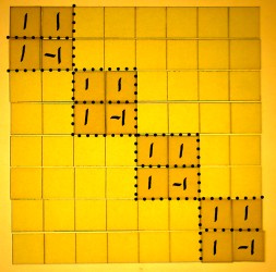
In this scheme the additions/subtractions are done before the
twiddling. Now I choose the first stage for illustration. The twiddle
factors do not appear in their natural order. One would quickly guess
what happened to the order...
 |
 |
|
These were the four basic radix 2 FFT forms, illustrated for N=8.
Modifications of them are conceivable, for instance a phase reordering
inbetween each stage, to have input and output in natural order
directly.
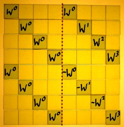
For convenience, the tables of the four schemes are showed once
more, next
to each other.
1. decimated spectrum:
|
|
|
|
2. decimated spectrum / decimated W series:
|
|
|
|
3. decimated input:
|
|
|
|
4. decimated input / decimated W series:
|
|
|
|