FFT in C

Now that I learned how a Fourier matrix can be decomposed into radix 2 FFT factors, the next challenge is to implement this in a computer language. After all, outside a computer even the optimallest Fast Fourier Transform is of little practical use. Although the first invention of the technique dates from the early nineteenth century...

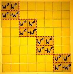
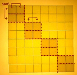
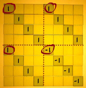
Below is the sketch of a radix 2 FFT for N=8, as it was figured out on preceding pages, and from which I will depart:

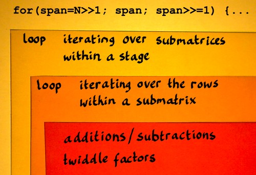
A routine for this FFT could or should be organised as a series of nested loops. I have seen this principle outlined in texts on FFT, notably in The Fast Fourier Transform by E. Oran Brigham, Numerical Recipes in C by William H. Press e.a., and Kevin 'fftguru' McGee's online FFT tutorial. The point is that I had a hard time to understand the mechanics of it. So I went step by step, studying texts and code, and working out my coloured square paper models in parallel. FFT was like a jig saw puzzle for me, and this page reflects how I was putting the pieces together.

In the matrix representation, the structure of an FFT shows several layers:

- the sparse factor matrices representing the FFT stages
- submatrices appearing in each factor matrix
- row entries appearing pairwise in each submatrix

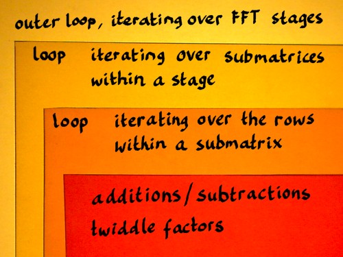
An FFT implementation can be organised accordingly, and for the moment I will just sketch that roughly:

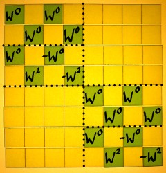
When we look at the FFT factor matrices, there is a kind of virtual vector size that is smaller and smaller in each consecutive stage. In the first stage, this size is N/2 and in the last stage it is reduced to just 1.

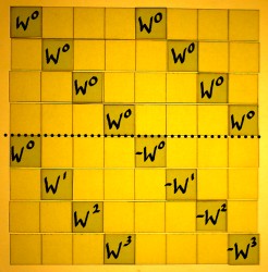
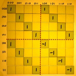
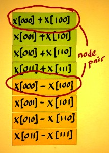
I feel that we should inspect the indexes in their binary form for a moment. Binary integer numbers are what computers use internally for indexing, which in turn is an incentive to do radix 2 FFT. If there is a pattern to perceive, it is best perceived in the binary numbers. Here is the addition/subtraction matrix of the first stage, with all indexes written in binary:

N/2 can also be defined N>>1, which means N shifted right by one bit: 1000 becomes 0100. It is a pure power of two everytime. Instead of using 4 as a constant, or writing N/2 a couple of times, it would be efficient to store the value in some variable, and update it in every stage. I will label this variable 'span', as that seems an appropriate title for this essential parameter.

We can declare span as a variable of datatype unsigned int, and initialize it at the start of the outer loop:

span = N>>1;

Span can be decremented in appropriate steps for the iterations over the FFT stages:

span >>= 1;

From 0100 it will shift to 0010 in the second stage and to 0001 in the third stage. After that it will shift right from 0001 to 0000, which is also boolean 'false'. That is where the outer loop should end indeed. Therefore the variable span can also regulate the conditions for the outer loop.

Let me insert this into the rough FFT sketch, in C manner:

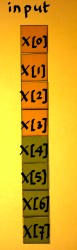
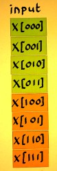
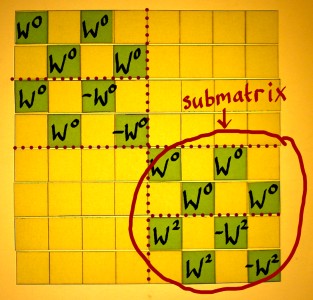
Index numbers can now be referenced as x[n] and x[n+span]. That is how we can identify sample pairs for addition/subtraction. This identification method will only run smooth when the work will be done on one submatrix at a time, within each stage. Otherwise x[n] will overlap with x[n+span]. We could write a for-loop that iterates over the submatrices in a stage.

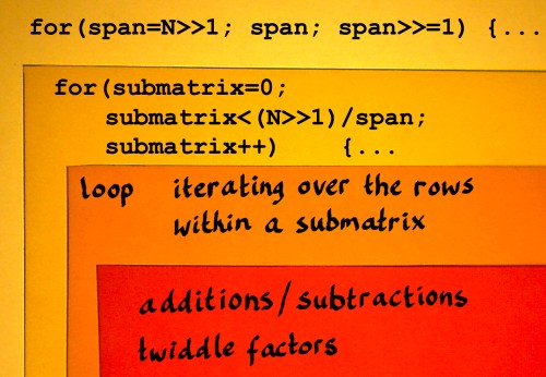
Every stage has it's own amount of submatrices. The first stage has just one NxN matrix. The second stage shows two submatrices. The third stage has four submatrices. The amount of submatrices in each stage is inversely proportional to span. More precisely, it is N/(span*2) or (N>>1)/span. Our for-loop can be something like:

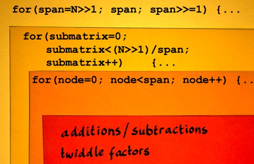
Adding these considerations to the FFT plan:

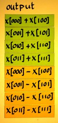
Within each submatrix we have to perform addition/subtraction and compute output pairs of the following kind:

I have seen such pairs being called 'dual node pairs', in Oran Brigham's book 'the Fast Fourier Transform'. There, the term applies to points where things come together in a butterfly figure. There is no butterflies here, but I like the term. Let me identify such a dual node pair like it shall be computed in the first FFT stage:

We bring x[000] and x[100] together, and perform addition of these on one hand, and subtraction on the other hand. After that, the results go their own way again.

How many dual node pairs do we have in a submatrix? There is already a variable that has the correct value: span. We can iterate over the dual node pairs using a straightforward loop that I will add to my preliminary scheme:

After finishing the iterations over the nodes, n has to jump over the x[n+span] values. But it must not get bigger than N. It can be done like: n=(n+span)&(N-1). The &(N-1) is a bitwise-and mask, for example: binary 11111 is such a mask in the N=32 case.

Until here I have three for-loops written down, but all the work of calculating the content still has to be done. What a crazy routine it is... Let me then see how to handle the additions/subtractions of the dual node pairs:

Aha. Here is a small problem: in this way the original value of x[n] can not be used for the computation of x[n+span], as it is already overwritten in the first line. Unfortunately, a temporary variable is needed to store the new value for x[n] for a short while:

This is all still quite theoretical, because x[n] is a complex variable in real life. Let us split x[n] in real[n] and im[n] for the moment, and check how the code could expand:

Now it turns out that for each n, the value [n+span] is already computed six times. Shall I not store this value before the additions and subtractions, in a variable called nspan? (Yep).

What comes next? We need to multiply the x[nspan] output values with twiddle factors. This is best done while these output values are still at hand, in the CPU registers (hopefully) or else somewhere nearby in cache. The twiddling is therefore inside the loop over the nodes, the innerest loop. Directly after the subtraction x[nspan]=x[n]-x[nspan], x[nspan] can be updated with the twiddle factor. Again, this is somewhat more complicated in real life, as it concerns a complex multiplication. And furthermore, we do not have these twiddle factors computed yet. So here I really have to start a new topic.

Twiddling

The twiddle factors shall be square roots of unity and square roots thereof, etcetera, related to each stage. Our N=8 FFT starts with the eight-roots of unity. The angle in radians for the primitive eight-root of unity, the first interval, could be computed with -2pi/8. But we have this handy variable span, initialized at N/2 and updated for each FFT stage. Therefore, angle of the primitive root for each stage can be computed as: -pi/span. So span functions as a complex root extractor, cool... This primitive root angle has to be updated for each new iteration within the outer loop:

If this root angle is multiplied with the node variable in the innerest loop, we have the correct angle for every twiddle factor:

From this angle, sine and cosine must be computed. That could simply be done like:

I will postpone my comments on this till later, let me first try to finish the routine. real[nspan] and im[nspan] need complex multiplication with realtwiddle and imtwiddle. Again, a temporary variable is inevitable:

For the next node, n must be incremented. We're done! Let me now put these codebits together.

With some twenty lines of C code we can have an FFT function. The output of this FFT appears in bit-reversed order, so for analysis purposes it does not make much sense yet. I will figure out bitreversal on a separate page. Furthermore, the output is not normalised in any way.

Of course, this simple FFT code is still highly inefficient. The real killer is: the calling of standard trigonometrics, cos() and sin(). Why is that so? For one thing, the hardware FPU trig instructions generate 80 bits precision output by default. They really take a lot of clock cycles. If we are to optimize the code, here is the obvious point to start. The next page shows some modifications.