Chirp Z Mechanism

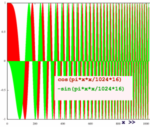
After doing a couple of tests with chirp Z transform, like zooming in on the spectrum and resampling, I became more and more intrigued by the method. It is hard to imagine how it works, or even why it works. I decided to follow the process step by step, with help of plots.

Below, a complex linear chirp is plotted. It has a negative rotation because of the minus sine part. The apparent speeding up is caused by the squared index. It is not so speedy as it could have been, without the zoom factor 16. I picked this factor to have a clearer plot for the moment.

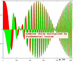
When a signal is fed into chirp Z transform, the first thing that must happen is multiplication with the chirp. But you could also state that the chirp functions are modulated by the input. I did an example with a fundamental cosine. The chirp functions are amplitude modulated and have their sign flipped over the center range.

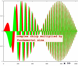
For comparison I did the same thing with a fundamental sine as the input signal. The second half of the chirp is now sign-flipped.

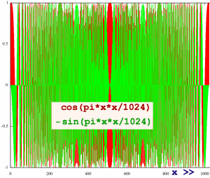
Now I want to check a 'full chirp', one that does not zoom. The chirp seems to speed up till the center of the frame and then speed down towards the end. But all instantaneous frequencies have negative sign, and keep growing in the absolute sense. Over the interval x[1024]-x[1023] it is almost -2pi. There is no u-turn point.

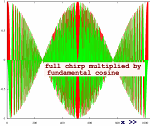
The full chirp modulated by the fundamental cosine gives:

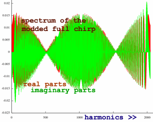
This modulated chirp must now be analysed with an FFT of larger framesize, since we are going to do fast convolution. The resulting spectrum looks remarkably similar to the signal. That is no coincidence, because the chirp frequency localisations in time domain are related to their localisations in frequency domain.

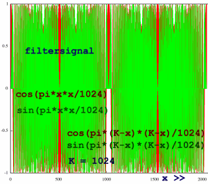
This spectrum has to be multiplied by the spectrum of chirp Z's filterkernel. The filter stretches over the length of input plus output of the transform, as was described on my chirp Z intro page. I have set outputsize = inputsize = 1024 for this case, so filter length is 2048. In time domain, it looks like this:

The spectrum of the double chirp, is chirp-like again:

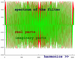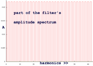
A full chirp has a perfectly flat amplitude spectrum, but here are two smaller chirps in one FFT frame. Checking part of it's amplitude spectrum, it turns out that every other bin has correlation zero.

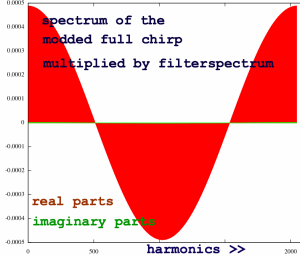
A surprise comes when the complex multiplication of modulated input spectrum with filter spectrum is done. All those dizzying chirp rotations are undone! Almost. Seems like we have our input fundamental cosine here.

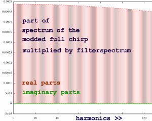
Of course, this cosine is also diluted with zero's:

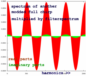
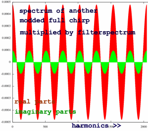
If I feed a cosine of periodicity 4 or 8 into the transform instead of the fundamental, the pattern is similar, except for the real/imaginary parts ratio:

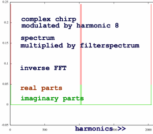
The next step in chirp Z transform is IFFT, to fulfill the fast convolution. Below, I did that for the case of cosine harmonic 8 as input. At last, we have something that looks like a spectrum of a cosine. Because of all the zero's, there is correlation near Nyquist frequency.

But of this output, only 1024 points are relevant since that is the outputsize.  The second half of the 2048 point output is 'scrap samples', as it results from semi-circular fast convolution. The tranform is not complete yet, one more rotation with a complex chirp has to be done. After all those spectacular metamorphoses, we get this dull output:

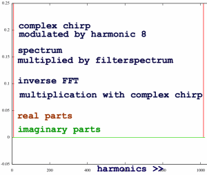This transform is equal to a regular 1024 point FFT, except half of the correlation weight is lost in the convolution. And it took ten times more CPU time.

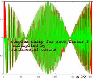
Now I am going to do a case with zoom factor 2. The input is the fundamental cosine again. Below you see the product of cosine and chirp. Notice that the chirp is slower, it goes till Nyquist.

Analysed with a double size FFT, it gives this spectrum plotted below. In fact, the downsampled cosine already appears here, in a crude form.

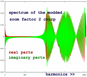After multiplication with the filterspectrum, which is now also modified for zoom factor 2, the following shape results:

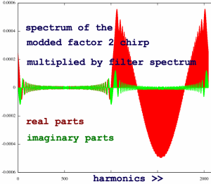It still looks heavily distorted. Let us see what IFFT and final chirping will make of this:

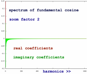Everything happens at the left side. Here is a detailed plot of that:

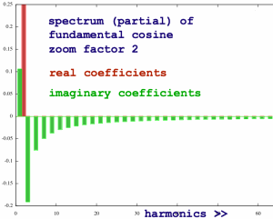The imaginary parts are mysterious. They indicate a phase shift, but in my resampling experiments I had not seen any phase shift. To confirm, let me revert the zoomed fundamental cosine to time domain with regular FFT. It is a pure cosine, of half the original length:

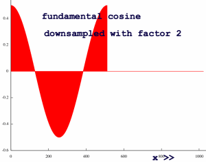I am curious about the role of the imaginary coefficents in this particular spectrum. Ha, they will not be able to keep their secret for long. I will just IFFT the real and imaginary coefficients separately, to see the individual contribution of both:

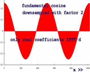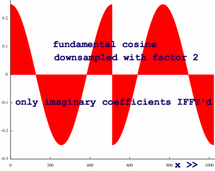Whah... imaginary coefficients can code cosines?! Though half of them upside down. This is the first time that I see a plot of a cosine-shaped, but still asymmetric waveshape. So the second half of the signal is effectively muted by cancellation.

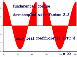
Let me also do a case with zoom factor 2.2. Again, the imaginary coefficients mute the real coefficients in the second part of the signal, while adding to the first part. But it is getting more mysterious... how come they both have a hole in the middle? Who is muting that part?

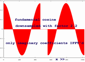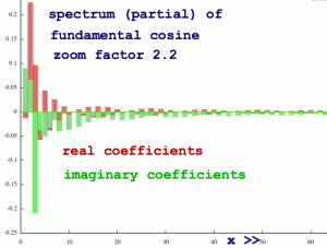
These holes are not result of real/imaginary cancellation. They are just coded in the patterns of real and imaginary coefficients themselves. All discrete time domain information, no matter what weird shape it has, can be stored in a spectrum of equal size. The first spectrum samples give an impression of how that is done for this particular case.

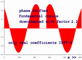
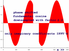
I need to verify what happens to a phase shifted input:

The zooming transform seems wonderfully precise. But now look what happens when zoom factor 1.5 is used. The 'tail' of the cancellation coefficients is missing. This introduces inaccuracies at the discontinuity locations:

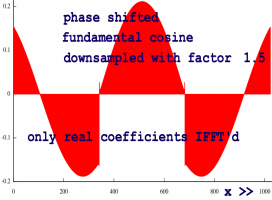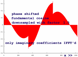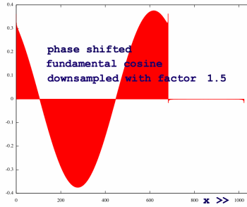
The resultant signal is (fortunately) only affected at the boundaries:

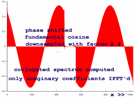
A similar effect is seen when we compute conjugates before resampling. This may be necessary to avoid to eliminate aliases in the negative frequencies range, which we do not want in the signal:

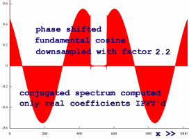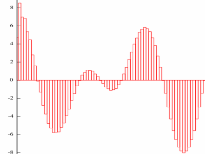
I copied a detailed plot of such a signal boundary from the page Resampling with Chirp Z.

Further research on this topic might reveal options to reduce these effects. But regular window and overlap may sufficiently relieve this problem in practical applications. For me, the main topic was to track the inner mechanism of chirp Z transform. I have seen a bit of that now. However, my quest is not fulfilled yet. I wanted to try a logarithmic chirp instead of linear, but I failed badly. Maybe some other time.