Bluestein and Chirp Z

While learning about Fourier Transform, I came across the rather enigmatic concept of chirp Z transform every now and then. I did not understand a bit of it, but since it was suggested that you could perform 'zoom FFT' with this technique, it seemed attractive. Now that I got more familiar with Fourier Transform after developing my own FFT library, I decided to take a closer look at chirp Z.

It can be stated that both Discrete Fourier Transform and chirp Z transform are specific cases of a more general principle, Z transform. Instead of trying to define Z transform here, which would probably lead me into trouble, I would like to illustrate in what sense chirp Z differs from Discrete Fourier Transform.

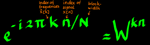
From the page Fourier Matrix I copied this formula of the forward DFT:

In this formula, the hatted x represents the Fourier Transform of a signal x[n]. Index k is the frequency index, an integer multiple of the fundamental in the transform framesize. Therefore, k are harmonics, though index zero, DC, is not a harmonic in the proper sense. All complex exponentials in the transform matrix are arranged in a square, with harmonics represented as row indexes k, and time direction as column indexes n. For ease of reading, the complex exponentials are abbreviated W^kn.

On this W^kn, a mathematical trick can be done to decouple the indexes. Chirp Z transform is an extension of 'Bluestein's algorithm' and Bluestein is the inventor of the trick. Wikipedia has an article on the topic. It is all about this identity:

With the product kn in the exponent of W replaced by three terms, the expression W^kn can be written as a product of three factors:

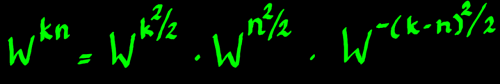After this factorisation, the transform formula can be reorganised. The first of the factors is not dependent on n, and is taken out of the summation:

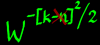
The summation result for each k must be multiplied with W^{(k^2)/2}. The signal x[n] can be multiplied with W^{(n^2)/2} before all other operations. But what to do with this weird W^{-((k-n)^2)/2}? It is the decisive part of the reorganisation. It makes the whole thing have the form of a convolution.

Making things complicated like this would not be so interesting if there were not fast convolution. Even then, what is the use of doing a transform as a convolution? As far as I understand, the original purpose was to decouple the n index from the k index and have free choice of lengths for the n and k arrays. In other words, the spectrum representation could have frequency intervals not dictated by the number of signal samples in the frame, or the FFT framesize. The technique was later expanded to make it even more flexible, and suitable for applications in diverse fields. Maybe I should better summarize Bluestein's algorithm in some scheme of operations, before going ahead.

It is quite a sequence of operations, and the output after doing step 7 for every k is just a spectrum. Notice that fast convolution is done as multiplication in frequency domain and the result is not obtained before doing inverse FFT. This is the point that I forgot when doing my first chirp Z attempts. Another important aspect is, that the arraylengths of input x[n] and output ẋ[k] plus one sample must together not exceed the length of the FFT frame used.

Since input length and output length are different, the complex chirps will also have different lengths. They are all based on W however, so their rate or speed will be the same. But how is W defined actually? Since neither input or output has the FFT framesize, what should be the basic interval or fundamental? It seems to me that the output length shall be the reference. Let me call this length K in accordance with index k. Then we have:

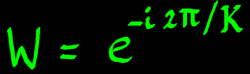And the chirp for the output goes:

The chirp for the input is similar. Although it's length is different, the rate or speed is determined by length K and not N. At least, that is what I think. I am not the type that will first read the complete chirp Z literature before implementing, and this is one of the things that I will have to check by experiment.

To have an impression of a complex linear chirp function, with it's squared indexes in the cos and sin arguments, I did the following plot:

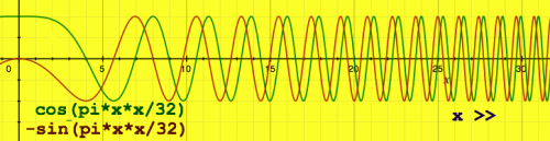By the way, what is so linear about this chirp? It's frequency or angular velocity is variable, but it's acceleration is constant, that must be the reason it is called linear. This in contrast with a logarithmic chirp, where the index is in the exponent of some base, like cos(2^x). The instantaneous frequency then has an exponential rise.

Multiplication of the signal x[n] with the chirp is straightforward. The signal may be real but the product is complex anyhow. This is fed into a complex forward FFT, but not before the values at indexes N and higher are set to zero. (N is the signal length, not the FFT length). Multiplying the complex output of the fast convolution with W^{(k^2)/2} is as simple.

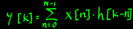
The factor W^{-((k-n)^2)/2} is more of a puzzle. A 'filter kernel' must be made, but how? The general formulation of convolution is:

Where h[k] is the filter kernel. In parallel to this, one could conclude that erasing the -n from our expression will render the filter kernel. Implemented like this, it should be a linear convolution, or not?

I tried it this way, but.... it does not work. Checking the chirp Z formula once more, I noticed the major difference with regular convolution: we are not computing outputs y[n] but y[k]. It looks more like this:

Which can also be written:

Or, specifying the k index range instead of the n index range:

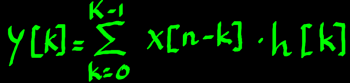It is as if the signal and filter have swapped their roles. Where you normally have the convolution output as a signal, running theoretically from minus to plus infinity, and in practice within length N+K-1, all relevant information must now go in length K. This can not be done as a linear convolution. It is more reminiscent of the overlap-scrap method, where you keep a segment of the output and scrap the tail(s). But now it is the filter kernel that should have overlap, instead of the signal input.

I had no idea how to handle this matter. Fortunately I found samplecode on internet that helped me out. It is published by Simon Sirin on Embedded.com.

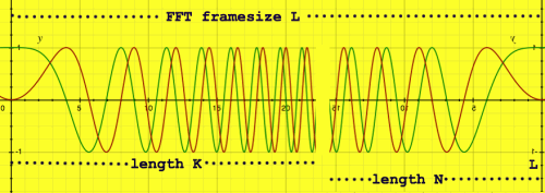
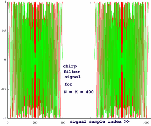
From that code I understand the following. The filter kernel must be extended leftward from time zero. Since the FFT is assumed to sample periodic waves, time L (L for framesize) is equivalent to time zero. Therefore 0-n = L-n. And (-n)² becomes (L-n)². There is nothing periodic about a chirp, but still this is the way to position it within the frame. Below is an impression. Notice that it is not for centered FFT. In case N+K-1 is smaller than L, there is still a zero-padded region inbetween the chirps.

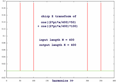
Now I can finally do an implementation of Bluestein's algorithm. This is not the 'zoom-FFT' yet; it is just doing this inputlength/outputlength conversion. I chose to convert from N = 385 to K = 640. The spectrum is then stretched by a factor 1.66. I fed cosine test functions in, of periodicity 50 and 100. The spectrum presents them at bin 83 and 166 respectively. That is precisely what it should be. Cool!

The coefficients do not show up as the clear-cut needles they would be after regular DFT. They are phase-shifted and pretty much smeared out. Is that the inevitable price of the translation? A sinusoid harmonically related to the input size, is inharmonic with the output size and vice versa. Therefore, cosines of any frequency result in the same smearing characteristic.

Of course, it is also possible to set output length equal to input length. Then those perfect needles can be produced again. This type of transform is useful for analyzing a signal that is clearly periodical, but not matching one of the radix 2 framesizes. With Bluestein's method, the framesize can be tuned to a signal's periodicity. That will produce a clearer analysis.

As usual, there is a normalisation issue. The input length is much smaller than the framesize so the sinusoids can not have their full magnitude that they would have otherwise. But is that the only effect?  Convolution is filtering, and in this case the filtering was done in frequency domain by the spectrum of a chirp. So let us have a look at that:

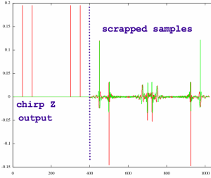
The chirp function is all complex exponentials, unit vectors. But there is a zero-padded region, which reduces the total energy. The filter spectrum was normalised with 1./FFTframesize in the forward transform. This reduces the energy seriously, but that loss is compensated in the inverse FFT. Probably the decisive loss is in the scrapped samples. Below, the scrapped output of the previous case is plotted together with the relevant part.

I am not going to settle this normalisation question now, because I want to try the 'zooming' options of chirp Z, and then conditions may be different again. But it certainly is an important topic.