Fast Convolution

From textbooks and classroom I have learned that convolution in time domain is equivalent to multiplication in frequency domain and vice versa. When using long impulse responses (filter kernels), multiplication in frequency domain can be the most efficient of the two methods. There is however this effect of convolution, that the output length equals the input signal length plus the filter kernel length, minus one sample. Therefore, a faithful translation of convolution to the frequency domain is not so straightforward. A plain multiplication of the signal's and filter's spectra will result in circular convolution. As a matrix operation, circular convolution can be sketched like this:

Compare this to linear convolution, like it is sketched below. If the linear convolution's tail is cut off and fold over the start, you get the circular convolution's pattern.

The only case where this would cause no problem, is with the filter being an identity matrix. It may also be a time-shifted identity. To verify this, I multiplied a signal's spectrum (of two cosines summed) with the spectrum of a time-shifted Kronecker delta. The output after inverse FFT shows the signal time-shifted indeed.

This is my first fast convolution: a wasteful method to delay a signal... But it is nice to have a pure example of delay implemented in frequency domain. Checking the output vertical scale, the amplitude appears reduced by a factor N, where N is the FFT framesize. The 'Kronecker filter' has it's amplitude spread over N frequency bins, since it was normalised with the same factor as the signal: 1/N in the forward transform. Though it is not a realistic case of fast convolution, it shows normalisation as a topic of consideration once more.

Now I want to fast-convolve two signal inputs of equal length, to check if it is true that the output signal will have the summed length of signal 1 and signal 2 (minus one sample). For simplicity, I choose two equal rectangular signals, each with half the FFT framesize. Because I have my FFT frame virtually centered round time zero, I need to center these input signals as well. The picture on the right below shows the spectrum of the a rectangular waveshape.

The spectra of two such rectangles are multiplied, with complex multiplication of course. That is actually a matter of computing the complex square of the spectrum. Then I feed the result in an inverse FFT. The output signal stretches over the frame indeed, and it has the shape that one could expect from two rectangles convolved. Still I find it kind of miraculous.

Next I did fast convolution of a similar rectangular signal with a chirp signal. Again, the resultant signal length is the sum of the input lengths.

The signal/filter inputs can have any length ratio, as long as their sum length does not exceed the FFT framesize plus one sample. Below is an example with a rectangular signal of 3/4 framesize and a chirp of 1/4 framesize.

The input/output length difference in convolution complicates matters even more when a long signal must be processed piecewise using fast convolution. If the input signal is cut in arrays of equal length, the bigger output arrays should overlap, and be summed to form the final output. Here is an impression of that:

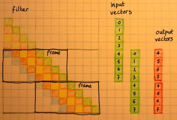
I have also tried to sketch the parallel with a time domain matrix. It is a case of framesize N=8. Four samples of the input are processed per N=8 frame, and the filter kernel has 5 samples. This yields an output y[n] of 8 samples everytime. When working in frequency domain, all vectors shall be transformed with a N=8 (I)FFT: input, filter kernel, output.

Below you can see how the output vectors of subsequent frames overlap. The first four samples in this example overlap with the preceding output, and the last four with the next output. Overlapping output means that values are to be summed. For this reason, the method is generally called 'overlap-add'. Notice that the overlap region is the length of the filter kernel minus one sample. So it need not be half the output vector length, but in my example it happens to be the case.

Instead of having the output arrays overlap, it is also possible to take overlapping segments of the input stream. You must then discard a portion of the output arrays, to get the correct result. Below I indicated the area of the matrix being skipped with this method. The number of output samples discarded equals the number of samples in the filter kernel minus one. 

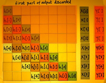Below, you can see what is actually processed in subsequent frames. The output portions are not summed, just cut clean and glued together. Which output samples shall be scrapped, is dependent on the position of the signal and the filter kernel within the FFT frame. In my case where everything is centered, it is the middle part that must be kept. With non-centered FFT it is different: normally the first part is scrapped, but by shifting the filter kernel the output position can be manipulated.

This method is sometimes and with good reason called 'overlap-discard' or 'overlap-scrap'. More often it is called 'overlap-save', because you need to save part of the input vector for the next frame. Using this method, the final output vector will be smaller than the total input vector. Theoretically, that is the wrong way round. The leading and trailing parts of the convolution are missing. If needed, the input vector can be extended on beforehand, at both ends, to make room for these transients.

My interest in fast convolution is specific: I want to try chirp z-transform, a technique which employs fast convolution to escape from the strict resolution grid of Fourier Transform. In that case, I might do some zero-phase filtering in frequency domain and deconvolve before IFFT. There would not be an overlap issue, but the rule of signal length + filter length + 1 not exceeding the framesize would still hold.