Inner Product

At the heart of digital signal processing is linear algebra, 'matrix algebra'. And at the heart of linear algebra is the inner product. Linear algebra is a huge area of research, most of of which I do not understand at all. Fortunately the inner product is a simple concept, and from there you can penetrate into deeper levels of the subject.

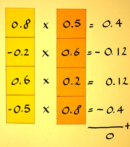
On a previous page I illustrated how matrix multiplication is a matter of cutting the things into rows and columns and find the correlations of these vectors. Here is a cut 'n paste from that page to refresh. The inner product is the sum of products of corresponding vector components. The result is one number that tells the measure of correlation between the vectors; how much they have in common.

Finding an inner product of vectors can serve various purposes:
- you want to analyse the correlation of the vectors
- or you want to manipulate the content of vectors

The correlation of two vectors can be a positive or negative number, or it can be zero. It can be a complex number too, in case the arrays are complex. Speaking of complex numbers: these have a special connexion to the concept of inner product. Let us take a close look at complex multiplication again. It is a simple but very significant process. Here is (a+ib)(c+id) in it's two equivalent matrix incarnations (yes, complex multiplication is commutative):

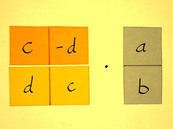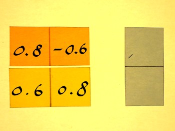
Choose an arbitrary example for (a+ib): (0.8+i0.6). Instead of doing the complex multiplication with (c+id), we will now inspect the content of the 2x2 matrix and calculate the inner product of it's rows.

It is zero. And it will be zero for the 2x2 multiplication matrix of any complex vector (a+ib). Apparently, during complex multiplication a complex vector is represented by two other vectors, and I will draw these to check what they look like:

(a-ib) is called the 'complex conjugate' of (a+ib). It is the reflection of (a+ib) over the x-axis. (b+ia) does not have a distinguished title like that. It is just ehm... the flip of (a+ib). Anyway, (a-ib) and (b+ia) are perpendicular vectors. They call that: orthogonal. And we have seen the inner product of these vectors: zero. Orthogonal vectors have inner product zero. The 2x2 matrix of complex multiplication is an orthogonal matrix, because the vectors in it are orthogonal.

While perpendicularity or orthogonality can be visualised for the case of vectors with two components, this is impossible for vectors of more than two components. From here on, we must extend the concept algebraically. The inner product tells the correlation of vectors, and a correlation of zero means orthogonality.

The question is: what does orthogonality 'look' like, for vectors with 2+ components? For vectors with an even number of components, it is quite easy to identify a vector perpendicular to it. Let us do an example with vector (a,b,c,d). First flip the vector, that means, present it time-reversed.

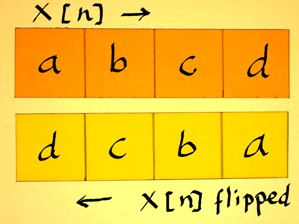The flipped vector must than be alternated, which means it is multiplied with 1 and -1 alternating. This can also be expressed as multiplication with (-1)ⁿ. Which is -1⁰, -1¹, -1² etcetera, assuming that indexing x[n] starts with n=0.

These vectors are orthogonal, no matter what values a b c and d have. Let us check this. Choose some arbitrary values for x[n] and alternate-flip the vector:

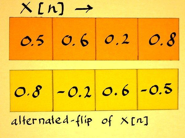Then compute the inner product:

The inner product is zero, so the vectors are orthogonal indeed. The alternate-the-flip method will work for any vector with an even number of components, no matter what it's values are. This could be applied to make orthogonal half-band filters. These may (and will) have overlap in frequency response, but because of the orthogonal filter arrays, the splitted signal is perfectly reconstructible.

Orthogonality is a big topic, and I will do a separate page on that. But first we have to inspect yet another feature of vectors: they have a 'length', comparable to complex vectors having a radius length. Such length is rather called 'norm', to indicate that it is more abstract than a fysical length. Furthermore, it is not the array length. So from here on I will speak of: vector norm.

The first step in computing the vector norm of x[n] is finding an inner product again. In this case, the inner product of x[n] and x[n] itself. Does that have a special name? I don't know. The inner-inner product?

Write the inner product of it:

Here we have a signal squared, x²[n]. It is equivalent to the total energy in a signal (though not in the stricter sense of alternating current, because we did not specify any DC-filtering).

The second step, which finally results in the vector norm, is finding the square root of the sum of squares:

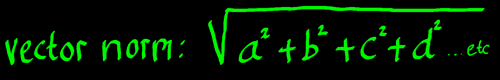That has a remarkable similarity to computing the radius length of a complex vector. A radius length is to be considered a vector norm as well. I tend to think of vector norm as 'Pythagoras extended'. Pythagoras extended to vectors with more than two components.

The above described vector norm is called: L² norm. Other norm-definitions are conceivable. For example, L³ norm would mean the cube root of the sum of cubes. But in linear algebra, we are computing inner products of two vectors at a time, not three vectors or whatever. Therefore the L² norm is the relevant norm.

Like complex numbers on the unit circle, all vectors with vector norm 1 are unit vectors. Unit vectors are of special importance, because they do not alter the norm of a target vector, in matrix multiplication. This may be a requirement in an operation, or if not, it may still be a reference point. Therefore, it is interesting to see how we can scale a vector with arbitrary norm to a unit vector. The procedure is said in a couple of words: divide the vector by it's norm. Let us do some simplistic examples to see the pattern in it. The first one is a complex vector (1+i1):

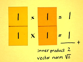The result is a complex number on the unit circle indeed, it is (cos(pi/4)+isin(pi/4)).

Next I will do a vector with four components (1,1,1,1):

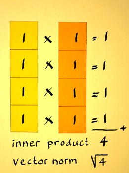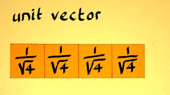Now compute the norm of this new vector to check if it is 1 indeed:

There are infinitely many unit vectors x[n] with four components of course. Everytime I seem to choose the trivialest of examples. But that is on purpose. The square-root-of-N arrangement, as it recurs in the examples, comes in handy when you need to append known unit vectors into larger arrays. Say you want to combine four arbitrary complex unit vectors into one new unit vector. No need to compute the norm of the whole thing first. Dividing all components by the square root of 4 will do the job. If you want to append eight unit vectors, divide all components by the square root of eight. Etcetera.