This page is not (at all) on 'peak to peak normalisation' like it is
done in wave editors. Instead, I want to discuss normalisation types
for sinusoid vectors in transform matrices. The vector norms have
decisive impact on the interpretation of the correlation output. Is the
output coefficient an amplitude? Or is it a (co)sine magnitude? It can
be
one of both, or even something else, depending on how you normalise.
Normalisation is not a very
popular topic in dsp textbooks. Admittedly, it is rather tedious
matter. But time and again confusion about normalisation has returned
on me, like a boomerang. I decided to sort it out in detail, with help
of plots and spreadsheets.
A square transform matrix contains N vectors, each with N
components. The page Fourier Matrix
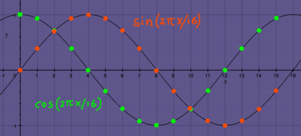
has pictures on that. Below I have sketched a sine and cosine vector,
both doing one cycle in
16 samplepoints x[n]. These vectors are the examples that we are going
to normalise. Notice that, while N=16, indexing starts at zero, so the
highest index number is 15.
 |
First I will check the vector norms as they are, without any
normalisation. Recall that a vector norm is computed with 'Pythagoras
extended'. First compute the sum of the values squared, which is an
inner product. Then take the square root of that, which is the norm.
 |
I computed the (co)sine values at all angles (2*pi*n/N). I squared
these values, and summed them to find the inner product. These vectors
have inner product 8. The square root of 8 is around 2.83, and that is
the norm.
 |
Pairs of sin(x) and cos(x) can be handled as a complex unit vector
of the general form cos(x)+isin(x).
Pointwise they always have amplitude 1 together. Two-point unit vectors
like these can subsequently be appended, using the normalisation factor:
 |
On the page Inner Product these things were illustrated with small
matrix examples. Now we can use the routine to append 16 complex unit
vectors and make a new unit vector of that. All the sine and cosine
values are multiplied by N-(1/2). The result gives norm
0.707107 for each phase. That is 2-1/2 or 0.51/2
of course.
 |
Together, the phases in the above spreadsheet are a unit vector:
 |
If a square matrix is filled with complex unit vectors, the
transpose of that matrix is the inverse. No further scaling is needed.
But, maybe you want a phase in itself to be a unit vector for some
reason. Imagine the case that you are not using complex vectors at all.
A cosine unit vector is found with an extra factor 21/2 to
the N-(1/2):
 |
See how easy it is to make unit vectors with (co)sines. If you have
a thousand-or-more-point vector, no need to compute the inner product
and the norm before you know how to normalise. Just use the known
factors.
I stated before that unit vectors in a (square) transform matrix
will preserve energy. Let us now check what happens if the unit cosine
vector from the above spreadsheet is used as a correlation vector in a
transform matrix, while the non-normalised cosine from the first
spreadsheet is the correlated input vector:
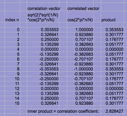 |
The norm of the correlated vector now appears as the correlation
coefficient. Below is a plot of this correlation process.
 |
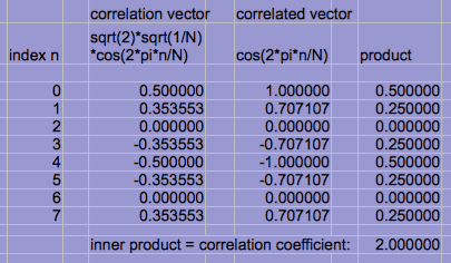
For different N, the coefficient reflecting a full cosine would
vary. Here is a sheet with N=8 to illustrate that:
 |
The preservation of energy may be beneficial in certain situations.
But to us, human observators, the coefficients do not make
much sense this way. When a transform is used for analysis purposes,
other types of normalisation can be used, to yield a more
comprehensible output. Let us consider a 1/N normalisation. The
spreadsheet below displays that 1/N will not make unit vectors:
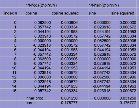 |
In fact, normalisation with 1/N is 'norma-normalisation', a double
normalisation. Because:
 |
Important: when using the factor 1/N in the transform, the
non-normalised vectors should be used in the inverse transform.
Otherwise you would norma-norma-norma-normalise. Which would result in
a very low output.
Let us now do correlation with a 1/N norma-normalised cosine vector,
and a full cosine as the input:
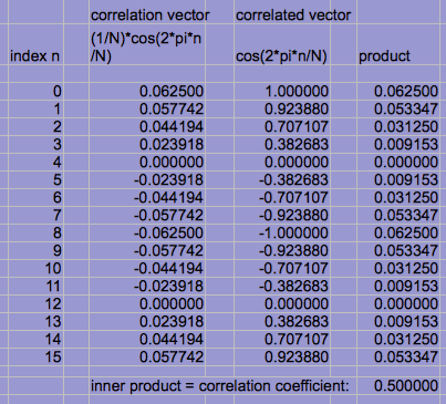 |
With 1/N normalisation, half of the cosine input is detected. The
reason for sinusoids detecting half the input was discussed in more
detail on the Sinusoids
Correlation page. If we would do a full complex
transform matrix, the other half would be found in the complex
conjugate part.
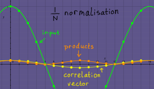
The 1/N normalisation for N=16 is illustrated below with a plot.
Compare with the earlier plot, where a unit cosine vector was used. The
correlation vector and the product values are much smaller now. For
larger N these differences become even more prominent.
 |
If we transform real signals only, computing conjugates could be a
waste of effort. When normalisation is done with 2/N, a cosine input is
fully detected in the correlation, as the next spreadsheet shows.
 |
With 2/N normalisation we will find the sine and cosine parts of
real signals directly in the correlation coefficients, without further
computations.
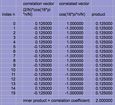
But now we stumble upon the exceptional cases of DC and
half-the-samplerate. In these cases, cosine has double energy and sine
has zero energy. On the other hand, they have no conjugates, and should
not be computed twice, like the others. If you do not make an exception
for them in the normalisation, you will detect twice the cosine that
actually went in. Now that I am doing all these spreadsheets, why not
illustrate the DC case as well. I am using the same 2/N normalisation
here for comparison:
 |
And here is cosine for the 'Nyquist case', the half-samplingrate
case:
 |
Till here we have seen how the coefficients can represent sine and
cosine magnitudes. But sometimes, the parameter of interest is the
amplitude for any of the frequencies. Here may be a pitfall
awaiting the confident engineer. Because, how do we normally compute a
radius or amplitude from real and imaginary part? With Pythagoras,
nothing can be simpler. But??? That does not represent the amplitude in
the signal. Then why is a radius called amplitude? Well it is an
amplitude actually, but of a two-point or two-phase vector. While we
were examining a one-phase signal, a real signal. To recompute the
two-point vector norm to a one point vector norm, we have to normalise
one more time with sqrt(1/N), where N=2. So with factor sqrt(1/2).
There is however an option to normalise in such a way that
coefficients reflect amplitudes per phase.
The normalisation factor is 21/2*(1/N). Here is the sheet of
such a case:
 |
I want to check if this really works as an amplitude correlator.
Here I put a 0.8*cosine vector in:
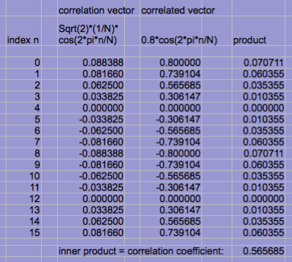 |
The result shows the amplitude that belongs to 0.8*cosine: 0.8*0.51/2=0.565685
indeed.
Notice that the DC and Nyquist exceptions exist here as well. Because
this is a 'reals only' normalisation again, neglecting the presence or
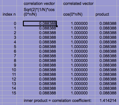
existence of conjugates. Look, this will happen to a DC input of
amplitude 1:
 |
Later, I found that it is pretty hazardous to make statements about
amplitudes, based on spectrum correlation coefficients. Because, what
the coefficients do not show you, is how components eventually
phase-cancel each other in time domain. Therefore, it may not be so
useful to know amplitudes at all.
After this spreadsheet overdose, still all is not said about
normalisation. I departed from the complex unit vector case, and
illustrated how you could do alternative normalisations of sine and
cosine phases, to have convenient coefficients for analysis. Employment
of sine and cosine in complex vectors is a typical aspect of Fourier
Transform. Other transform types, like Discrete Cosine Transform and
Wavelet Transform, demand their own normalisation considerations. These
matters must remain unclarified here, if only for the reason that I
have too little knowledge of it. The boomerang is still in the air.