Centered FFT Frame

On this page, I want to reorganise my FFT routines again. Why so? Till now, my FFT's correlate the input with functions over the interval [0, 1] of the fundamental cycle, or [0, 2pi] in radians. For an impression of that, here is a plot of the first 5 harmonic cosines over that interval:

Phase angles run from zero till 2pi here. This can be inconvenient. Spectrum coefficients are complex, and frequency bins are neighboring branches of the complex plane. Theoretically, the branch cut can be defined anywhere, but for practical purposes it is often defined between -pi and pi radians. That is on the negative real axis, from the origin to minus infinity.

The complex arctangent function in the standard C library has that range, to mention one important consideration. At least for the forward transform, it would be better to correlate over the interval [-0.5, 0.5] of the fundamental cycle, and thus have phase angles of the spectrum output between -pi and pi radians:

Since we have no negative-signed indexes in computer implementations, it seems that we need to right shift the functions over half an interval or pi radians. That is what I thought at first sight. But ooopps, small problem:

A time-shift has different phase-effects for each frequency. The odd harmonics must be shifted by an odd multiple of pi radians and the even harmonics by an even multiple of pi radians. That means the even harmonics should remain like they are, while the odd harmonics can be multiplied with -1. Then we get this:

That looks better. For the sine parts a similar modification holds. In the forward transform we normally have negative sine functions like these:

Shifting the virtual zero point to halfway the interval requires the even harmonic sine functions to be negative, and the odd harmonics positive:

I have copied a Fourier matrix from an earlier page, and cut&pasted a phase-centered version from it, which is on the right. Recall that the W^kn factors are complex exponentials e^-i2*pi*k*n/N.

It is essentially a matter of swapping the left and right halves of the matrix.  As you can see, the beautiful symmetry of the original Fourier matrix is lost in the phase-zero-centered version. The rows are no longer equal to the columns. Therefore, row permutations are needed for the transpose in the inverse transform. That is illustrated below. On the left is the normal transpose and on the right is the permutated version.

It is also possible to center both time input, and frequency output, in the forward transform. In that case, the matrix is it's own transpose again, apart from the rotation of the complex exponentials in the inverse transform, as is always the case. You have to get used to the rotated spectrum then. The positive frequencies appear in the upper half of the output.

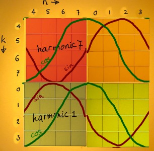
Since we are specially concerned with the behaviour of the odd harmonics, I want to sketch an impression of the impact on these. On the left below, two harmonics are sketched in a ordered Fourier situation, and on the right I centered the quarters according to input and output. Remarkably, the cosines flip but the sines do not. Still, taking the shifted spectrum into account, the relevant sine direction is flipped as well.

Fortunately, we do not need elaborate mathematical formula's to achieve these effects. There is only one mechanism at work. Multiplying the input with (-1)ⁿ will center the output. And centering the input will multiply the output with (-1)ⁿ. No matter what input: time signal or spectrum. So at both ends of the transform the same things happen. You can do both: center the input and multiply it with (-1)ⁿ. You then get an output which is centered and alternated as well. That is the effect of the Fourier matrix in the last figure. I went through quite some mishaps with code typo's and other errations before getting fully convinced of this simple truth.

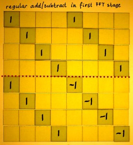
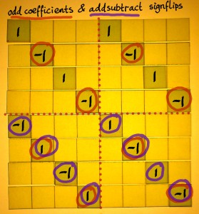
The centering and alternations can be done outside the FFT routine, but it is more efficient to integrate some sign-flippings in the first FFT stage.

Below is an illustration of that in my familiar square paper style so you can compare with my earlier FFT pages. Multiplication of the input array with (-1)ⁿ can be implemented as an adaptation of the first stage add/subtract factor matrix. The original is on the left and the adaptation on the right.

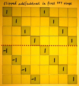
Centering the signal input, a virtual shift of time zero to the frame centre, is slightly less straigthforward. We have to sign-flip the odd correlation vectors in the FFT matrix. Basically, all odd harmonics in the FFT are 'inheritants' of the fundamental rotation, which is also odd. One option, of many, is to sign-flip the fundamental twiddle factors, both sine and cosine. All other twiddle factors are even harmonics and must be left untouched. Swapping the add/subtract factors is equal to sign-flipping the twiddles, so this again can be integrated in the same matrix, as shown on the left below. On the right is the combination of the two sign-flip actions.

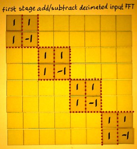
I found it even more convenient to do the modifications in an FFT scheme for decimated input. The first stage of that scheme has no twiddles, therefore it is advantageous to peel it anyway and do normalisation there. In a decimated sequence, the odd numbers and the highest half of the numbers in the array have their positions exchanged. On the page with bitreversal tables you can check which numbers go where in case of bitreversed permutation. It happens that similar sign-flipping actions can be done for this FFT scheme. On the left is the normal add/subtract factor matrix, and on the right the version that effectuates centering of the input.

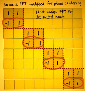To compensate for the phase/time-zero centering, the modification showed on the left below could be used in the inverse transform. Or both modifications can be combined in forward and inverse transform alike, as shown on the right.

Notice that an FFT for decimated input has a reversed sequence of operations, as compared to an FFT for decimated output. Four different FFT radix 2 schemes are illustrated on my page Radix 2 FFT Forms.

Let us now check the output of a forward FFT with time zero centered. I want to see if I get a familiar pattern when I enter a pulse at x[(N/2)+1], now being time one:

Indeed it is the same output that I had from a pulse at x[1] with my non-centered FFT. Apparently, the simple sign-flip does it's job well. I am curious how a pulse at x[33] would transform with a non-centered FFT, for comparison. Here it is:

The above plot illustrates the alternating spectrum, as it results from time-shifted input.

Now I return to the time zero centered input, and I want to combine with a frequency zero centered output. Harmonic zero (DC) is at index N/2 in this case. The spectrum is rotated. The benefit of this transform is a better symmetry between forward and inverse. But you have to remind this index offset, which may be inconvenient. I prefer not to make regular use of this representation.

Now that I know how to implement a virtual time-zero and/or frequency-zero centering, one dangling question remains. I have learned or at least concluded sometimes that multiplying a signal with (-1)ⁿ effectuates a 'rotation over pi radian' of the spectrum. On this page, I have carefully avoided that word, or replaced it by 'centered spectrum'. What does it actually mean, a rotated spectrum? In the plot above, the spectrum can be considered as being shifted rightward, while the part with negative frequencies is shifted in from the left. If you would make a circle of the x-axis over the range of the framesize, the shift would be a rotation over half the framesize. A circle... can we draw the spectrum on the complex plane? That is hard. To draw both phases and frequencies would require different branches of the complex plane in one figure.

Yet I want to produce some visualisation. Let me draw real and imaginary parts of a frequency as points with different colours. Then rotate the whole thing over half a circle. A low frequency becomes a high frequency. You get the alias(es). In addition to that, the negative frequencies become the positive frequencies and vice versa.

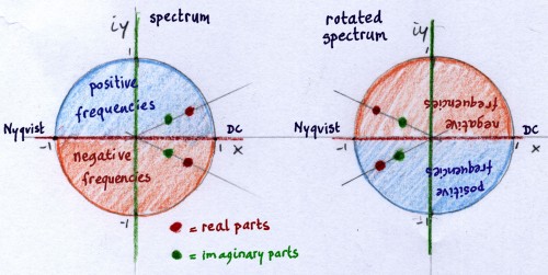If you would flip the signs of the imaginary parts to conjugate the spectrum, after rotation, you would get exactly the inverse of the original spectrum. Why would one create an inverse of a spectrum? It is an important aspect of Wavelet theory to create orthogonal halfband filters. I was just curious how I could visualize that, though it is quite off-topic here. In Wavelets technique, they do alternate-flip the filter impuls response: reverse the signal's direction and multiply with (-1)ⁿ. This is almost the equivalent to rotation and conjugation of the filter kernel's frequency response. Except for that one-sample discrepancy you get when time-reversing a discrete signal. (See the page Invertible FFT).